Pyomo Documentation 6.8.0

Pyomo is a Python-based, open-source optimization modeling language with a diverse set of optimization capabilities.

Installation

Pyomo currently supports the following versions of Python:

• CPython: 3.8, 3.9, 3.10, 3.11, 3.12

• PyPy: 3

At the time of the first Pyomo release after the end-of-life of a minor Python version, Pyomo will remove testing for that Python version.

Using CONDA

We recommend installation with conda, which is included with the Anaconda distribution of Python. You can install Pyomo in your system Python installation by executing the following in a shell:

conda install -c conda-forge pyomo

Optimization solvers are not installed with Pyomo, but some open source optimization solvers can be installed with conda as well:

conda install -c conda-forge ipopt glpk

Using PIP

The standard utility for installing Python packages is pip. You can install Pyomo in your system Python installation by executing the following in a shell:

pip install pyomo

Conditional Dependencies

Extensions to Pyomo, and many of the contributions in pyomo.contrib, often have conditional dependencies on a variety of third-party Python packages including but not limited to: matplotlib, networkx, numpy, openpyxl, pandas, pint, pymysql, pyodbc, pyro4, scipy, sympy, and xlrd.

A full list of conditional dependencies can be found in Pyomo’s setup.py and displayed using:

python setup.py dependencies --extra optional

Pyomo extensions that require any of these packages will generate an error message for missing dependencies upon use.

When using pip, all conditional dependencies can be installed at once using the following command:

pip install 'pyomo[optional]'

When using conda, many of the conditional dependencies are included with the standard Anaconda installation.

You can check which Python packages you have installed using the command conda list or pip list. Additional Python packages may be installed as needed.

Installation with Cython

Users can opt to install Pyomo with cython initialized.

Note

This can only be done via pip or from source.

Via pip:

pip install pyomo --global-option="--with-cython"

From source (recommended for advanced users only):

git clone https://github.com/Pyomo/pyomo.git
cd pyomo
python setup.py install --with-cython

Citing Pyomo

Pyomo

Bynum, Michael L., Gabriel A. Hackebeil, William E. Hart, Carl D. Laird, Bethany L. Nicholson, John D. Siirola, Jean-Paul Watson, and David L. Woodruff. Pyomo - Optimization Modeling in Python, 3rd Edition. Springer, 2021.

Hart, William E., Jean-Paul Watson, and David L. Woodruff. “Pyomo: modeling and solving mathematical programs in Python.” Mathematical Programming Computation 3, no. 3 (2011): 219-260.

PySP

Watson, Jean-Paul, David L. Woodruff, and William E. Hart. “PySP: modeling and solving stochastic programs in Python.” Mathematical Programming Computation 4, no. 2 (2012): 109-149.

Pyomo Overview

Mathematical Modeling

This section provides an introduction to Pyomo: Python Optimization Modeling Objects. A more complete description is contained in the [PyomoBookIII] book. Pyomo supports the formulation and analysis of mathematical models for complex optimization applications. This capability is commonly associated with commercially available algebraic modeling languages (AMLs) such as [AMPL], [AIMMS], and [GAMS]. Pyomo’s modeling objects are embedded within Python, a full-featured, high-level programming language that contains a rich set of supporting libraries.

Modeling is a fundamental process in many aspects of scientific research, engineering and business. Modeling involves the formulation of a simplified representation of a system or real-world object. Thus, modeling tools like Pyomo can be used in a variety of ways:

• Explain phenomena that arise in a system,

• Make predictions about future states of a system,

• Assess key factors that influence phenomena in a system,

• Identify extreme states in a system, that might represent worst-case scenarios or minimal cost plans, and

• Analyze trade-offs to support human decision makers.

Mathematical models represent system knowledge with a formalized language. The following mathematical concepts are central to modern modeling activities:

Variables

Variables represent unknown or changing parts of a model (e.g., whether or not to make a decision, or the characteristic of a system outcome). The values taken by the variables are often referred to as a solution and are usually an output of the optimization process.

Parameters

Parameters represents the data that must be supplied to perform the optimization. In fact, in some settings the word data is used in place of the word parameters.

Relations

These are equations, inequalities or other mathematical relationships that define how different parts of a model are connected to each other.

Goals

These are functions that reflect goals and objectives for the system being modeled.

The widespread availability of computing resources has made the numerical analysis of mathematical models a commonplace activity. Without a modeling language, the process of setting up input files, executing a solver and extracting the final results from the solver output is tedious and error-prone. This difficulty is compounded in complex, large-scale real-world applications which are difficult to debug when errors occur. Additionally, there are many different formats used by optimization software packages, and few formats are recognized by many optimizers. Thus the application of multiple optimization solvers to analyze a model introduces additional complexities.

Pyomo is an AML that extends Python to include objects for mathematical modeling. [PyomoBookI], [PyomoBookII], [PyomoBookIII], and [PyomoJournal] compare Pyomo with other AMLs. Although many good AMLs have been developed for optimization models, the following are motivating factors for the development of Pyomo:

• Open Source

  Pyomo is developed within Pyomo’s open source project to promote transparency of the modeling framework and encourage community development of Pyomo capabilities.

• Customizable Capability

  Pyomo supports a customizable capability through the extensive use of plug-ins to modularize software components.

• Solver Integration

  Pyomo models can be optimized with solvers that are written either in Python or in compiled, low-level languages.

• Programming Language

  Pyomo leverages a high-level programming language, which has several advantages over custom AMLs: a very robust language, extensive documentation, a rich set of standard libraries, support for modern programming features like classes and functions, and portability to many platforms.

Overview of Modeling Components and Processes

Pyomo supports an object-oriented design for the definition of optimization models. The basic steps of a simple modeling process are:

• Create model and declare components

• Instantiate the model

• Apply solver

• Interrogate solver results

In practice, these steps may be applied repeatedly with different data or with different constraints applied to the model. However, we focus on this simple modeling process to illustrate different strategies for modeling with Pyomo.

A Pyomo model consists of a collection of modeling components that define different aspects of the model. Pyomo includes the modeling components that are commonly supported by modern AMLs: index sets, symbolic parameters, decision variables, objectives, and constraints. These modeling components are defined in Pyomo through the following Python classes:

Set

set data that is used to define a model instance

Param

parameter data that is used to define a model instance

Var

decision variables in a model

Objective

expressions that are minimized or maximized in a model

Constraint

constraint expressions that impose restrictions on variable values in a model

Abstract Versus Concrete Models

A mathematical model can be defined using symbols that represent data values. For example, the following equations represent a linear program (LP) to find optimal values for the vector \(x\) with parameters \(n\) and \(b\), and parameter vectors \(a\) and \(c\):

\begin{array}{lll} \min & \sum_{j=1}^n c_j x_j &\\ \mathrm{s.t.} & \sum_{j=1}^n a_{ij} x_j \geq b_i & \forall i = 1 \ldots m\\ & x_j \geq 0 & \forall j = 1 \ldots n \end{array}

Note

As a convenience, we use the symbol \(\forall\) to mean “for all” or “for each.”

We call this an abstract or symbolic mathematical model since it relies on unspecified parameter values. Data values can be used to specify a model instance. The AbstractModel class provides a context for defining and initializing abstract optimization models in Pyomo when the data values will be supplied at the time a solution is to be obtained.

In many contexts, a mathematical model can and should be directly defined with the data values supplied at the time of the model definition. We call these concrete mathematical models. For example, the following LP model is a concrete instance of the previous abstract model:

\begin{array}{ll} \min & 2 x_1 + 3 x_2\\ \mathrm{s.t.} & 3 x_1 + 4 x_2 \geq 1\\ & x_1, x_2 \geq 0 \end{array}

The ConcreteModel class is used to define concrete optimization models in Pyomo.

Note

Python programmers will probably prefer to write concrete models, while users of some other algebraic modeling languages may tend to prefer to write abstract models. The choice is largely a matter of taste; some applications may be a little more straightforward using one or the other.

Simple Models

A Simple Concrete Pyomo Model

It is possible to get the same flexible behavior from models declared to be abstract and models declared to be concrete in Pyomo; however, we will focus on a straightforward concrete example here where the data is hard-wired into the model file. Python programmers will quickly realize that the data could have come from other sources.

Given the following model from the previous section:

\begin{array}{ll} \min & 2 x_1 + 3 x_2\\ \mathrm{s.t.} & 3 x_1 + 4 x_2 \geq 1\\ & x_1, x_2 \geq 0 \end{array}

This can be implemented as a concrete model as follows:

import pyomo.environ as pyo

model = pyo.ConcreteModel()

model.x = pyo.Var([1,2], domain=pyo.NonNegativeReals)

model.OBJ = pyo.Objective(expr = 2*model.x[1] + 3*model.x[2])

model.Constraint1 = pyo.Constraint(expr = 3*model.x[1] + 4*model.x[2] >= 1)

Although rule functions can also be used to specify constraints and objectives, in this example we use the expr option that is available only in concrete models. This option gives a direct specification of the expression.

A Simple Abstract Pyomo Model

We repeat the abstract model from the previous section:

\begin{array}{lll} \min & \sum_{j=1}^n c_j x_j &\\ \mathrm{s.t.} & \sum_{j=1}^n a_{ij} x_j \geq b_i & \forall i = 1 \ldots m\\ & x_j \geq 0 & \forall j = 1 \ldots n \end{array}

One way to implement this in Pyomo is as shown as follows:

import pyomo.environ as pyo

model = pyo.AbstractModel()

model.m = pyo.Param(within=pyo.NonNegativeIntegers)
model.n = pyo.Param(within=pyo.NonNegativeIntegers)

model.I = pyo.RangeSet(1, model.m)
model.J = pyo.RangeSet(1, model.n)

model.a = pyo.Param(model.I, model.J)
model.b = pyo.Param(model.I)
model.c = pyo.Param(model.J)

# the next line declares a variable indexed by the set J
model.x = pyo.Var(model.J, domain=pyo.NonNegativeReals)

def obj_expression(m):
    return pyo.summation(m.c, m.x)

model.OBJ = pyo.Objective(rule=obj_expression)

def ax_constraint_rule(m, i):
    # return the expression for the constraint for i
    return sum(m.a[i,j] * m.x[j] for j in m.J) >= m.b[i]

# the next line creates one constraint for each member of the set model.I
model.AxbConstraint = pyo.Constraint(model.I, rule=ax_constraint_rule)

Note

Python is interpreted one line at a time. A line continuation character, \ (backslash), is used for Python statements that need to span multiple lines. In Python, indentation has meaning and must be consistent. For example, lines inside a function definition must be indented and the end of the indentation is used by Python to signal the end of the definition.

We will now examine the lines in this example. The first import line is required in every Pyomo model. Its purpose is to make the symbols used by Pyomo known to Python.

import pyomo.environ as pyo

The declaration of a model is also required. The use of the name model is not required. Almost any name could be used, but we will use the name model in most of our examples. In this example, we are declaring that it will be an abstract model.

model = pyo.AbstractModel()

We declare the parameters \(m\) and \(n\) using the Pyomo Param component. This component can take a variety of arguments; this example illustrates use of the within option that is used by Pyomo to validate the data value that is assigned to the parameter. If this option were not given, then Pyomo would not object to any type of data being assigned to these parameters. As it is, assignment of a value that is not a non-negative integer will result in an error.

model.m = pyo.Param(within=pyo.NonNegativeIntegers)
model.n = pyo.Param(within=pyo.NonNegativeIntegers)

Although not required, it is convenient to define index sets. In this example we use the RangeSet component to declare that the sets will be a sequence of integers starting at 1 and ending at a value specified by the the parameters model.m and model.n.

model.I = pyo.RangeSet(1, model.m)
model.J = pyo.RangeSet(1, model.n)

The coefficient and right-hand-side data are defined as indexed parameters. When sets are given as arguments to the Param component, they indicate that the set will index the parameter.

model.a = pyo.Param(model.I, model.J)
model.b = pyo.Param(model.I)
model.c = pyo.Param(model.J)

The next line that is interpreted by Python as part of the model declares the variable \(x\). The first argument to the Var component is a set, so it is defined as an index set for the variable. In this case the variable has only one index set, but multiple sets could be used as was the case for the declaration of the parameter model.a. The second argument specifies a domain for the variable. This information is part of the model and will passed to the solver when data is provided and the model is solved. Specification of the NonNegativeReals domain implements the requirement that the variables be greater than or equal to zero.

# the next line declares a variable indexed by the set J
model.x = pyo.Var(model.J, domain=pyo.NonNegativeReals)

Note

In Python, and therefore in Pyomo, any text after pound sign is considered to be a comment.

In abstract models, Pyomo expressions are usually provided to objective and constraint declarations via a function defined with a Python def statement. The def statement establishes a name for a function along with its arguments. When Pyomo uses a function to get objective or constraint expressions, it always passes in the model (i.e., itself) as the the first argument so the model is always the first formal argument when declaring such functions in Pyomo. Additional arguments, if needed, follow. Since summation is an extremely common part of optimization models, Pyomo provides a flexible function to accommodate it. When given two arguments, the summation() function returns an expression for the sum of the product of the two arguments over their indexes. This only works, of course, if the two arguments have the same indexes. If it is given only one argument it returns an expression for the sum over all indexes of that argument. So in this example, when summation() is passed the arguments m.c, m.x it returns an internal representation of the expression \(\sum_{j=1}^{n}c_{j} x_{j}\).

def obj_expression(m):
    return pyo.summation(m.c, m.x)

To declare an objective function, the Pyomo component called Objective is used. The rule argument gives the name of a function that returns the objective expression. The default sense is minimization. For maximization, the sense=pyo.maximize argument must be used. The name that is declared, which is OBJ in this case, appears in some reports and can be almost any name.

model.OBJ = pyo.Objective(rule=obj_expression)

Declaration of constraints is similar. A function is declared to generate the constraint expression. In this case, there can be multiple constraints of the same form because we index the constraints by \(i\) in the expression \(\sum_{j=1}^n a_{ij} x_j \geq b_i \;\;\forall i = 1 \ldots m\), which states that we need a constraint for each value of \(i\) from one to \(m\). In order to parametrize the expression by \(i\) we include it as a formal parameter to the function that declares the constraint expression. Technically, we could have used anything for this argument, but that might be confusing. Using an i for an \(i\) seems sensible in this situation.

def ax_constraint_rule(m, i):
    # return the expression for the constraint for i
    return sum(m.a[i,j] * m.x[j] for j in m.J) >= m.b[i]

Note

In Python, indexes are in square brackets and function arguments are in parentheses.

In order to declare constraints that use this expression, we use the Pyomo Constraint component that takes a variety of arguments. In this case, our model specifies that we can have more than one constraint of the same form and we have created a set, model.I, over which these constraints can be indexed so that is the first argument to the constraint declaration. The next argument gives the rule that will be used to generate expressions for the constraints. Taken as a whole, this constraint declaration says that a list of constraints indexed by the set model.I will be created and for each member of model.I, the function ax_constraint_rule will be called and it will be passed the model object as well as the member of model.I

# the next line creates one constraint for each member of the set model.I
model.AxbConstraint = pyo.Constraint(model.I, rule=ax_constraint_rule)

In the object oriented view of all of this, we would say that model object is a class instance of the AbstractModel class, and model.J is a Set object that is contained by this model. Many modeling components in Pyomo can be optionally specified as indexed components: collections of components that are referenced using one or more values. In this example, the parameter model.c is indexed with set model.J.

In order to use this model, data must be given for the values of the parameters. Here is one file that provides data (in AMPL “.dat” format).

# one way to input the data in AMPL format
# for indexed parameters, the indexes are given before the value

param m := 1 ;
param n := 2 ;

param a :=
1 1 3
1 2 4
;

param c:=
1 2
2 3
;

param b := 1 1 ;

There are multiple formats that can be used to provide data to a Pyomo model, but the AMPL format works well for our purposes because it contains the names of the data elements together with the data. In AMPL data files, text after a pound sign is treated as a comment. Lines generally do not matter, but statements must be terminated with a semi-colon.

For this particular data file, there is one constraint, so the value of model.m will be one and there are two variables (i.e., the vector model.x is two elements long) so the value of model.n will be two. These two assignments are accomplished with standard assignments. Notice that in AMPL format input, the name of the model is omitted.

param m := 1 ;
param n := 2 ;

There is only one constraint, so only two values are needed for model.a. When assigning values to arrays and vectors in AMPL format, one way to do it is to give the index(es) and the the value. The line 1 2 4 causes model.a[1,2] to get the value 4. Since model.c has only one index, only one index value is needed so, for example, the line 1 2 causes model.c[1] to get the value 2. Line breaks generally do not matter in AMPL format data files, so the assignment of the value for the single index of model.b is given on one line since that is easy to read.

param a :=
 1 1 3
 1 2 4
 ;

 param c:=
 1 2
 2 3
 ;

 param b := 1 1 ;

Symbolic Index Sets

When working with Pyomo (or any other AML), it is convenient to write abstract models in a somewhat more abstract way by using index sets that contain strings rather than index sets that are implied by \(1,\ldots,m\) or the summation from 1 to \(n\). When this is done, the size of the set is implied by the input, rather than specified directly. Furthermore, the index entries may have no real order. Often, a mixture of integers and indexes and strings as indexes is needed in the same model. To start with an illustration of general indexes, consider a slightly different Pyomo implementation of the model we just presented.

#  ___________________________________________________________________________
#
#  Pyomo: Python Optimization Modeling Objects
#  Copyright (c) 2008-2024
#  National Technology and Engineering Solutions of Sandia, LLC
#  Under the terms of Contract DE-NA0003525 with National Technology and
#  Engineering Solutions of Sandia, LLC, the U.S. Government retains certain
#  rights in this software.
#  This software is distributed under the 3-clause BSD License.
#  ___________________________________________________________________________

# abstract2.py


from pyomo.environ import *

model = AbstractModel()

model.I = Set()
model.J = Set()

model.a = Param(model.I, model.J)
model.b = Param(model.I)
model.c = Param(model.J)

# the next line declares a variable indexed by the set J
model.x = Var(model.J, domain=NonNegativeReals)


def obj_expression(model):
    return summation(model.c, model.x)


model.OBJ = Objective(rule=obj_expression)


def ax_constraint_rule(model, i):
    # return the expression for the constraint for i
    return sum(model.a[i, j] * model.x[j] for j in model.J) >= model.b[i]


# the next line creates one constraint for each member of the set model.I
model.AxbConstraint = Constraint(model.I, rule=ax_constraint_rule)

To get the same instantiated model, the following data file can be used.

# abstract2a.dat AMPL format

set I := 1 ;
set J := 1 2 ;

param a :=
1 1 3
1 2 4
;

param c:=
1 2
2 3
;

param b := 1 1 ;

However, this model can also be fed different data for problems of the same general form using meaningful indexes.

# abstract2.dat AMPL data format

set I := TV Film ;
set J := Graham John Carol ;

param a :=
TV  Graham 3
TV John 4.4
TV Carol 4.9
Film Graham 1
Film John 2.4
Film Carol 1.1
;

param c := [*]
 Graham 2.2
 John 3.1416
 Carol 3
;

param b := TV 1 Film 1 ;

Solving the Simple Examples

Pyomo supports modeling and scripting but does not install a solver automatically. In order to solve a model, there must be a solver installed on the computer to be used. If there is a solver, then the pyomo command can be used to solve a problem instance.

Suppose that the solver named glpk (also known as glpsol) is installed on the computer. Suppose further that an abstract model is in the file named abstract1.py and a data file for it is in the file named abstract1.dat. From the command prompt, with both files in the current directory, a solution can be obtained with the command:

pyomo solve abstract1.py abstract1.dat --solver=glpk

Since glpk is the default solver, there really is no need specify it so the --solver option can be dropped.

Note

There are two dashes before the command line option names such as solver.

To continue the example, if CPLEX is installed then it can be listed as the solver. The command to solve with CPLEX is

pyomo solve abstract1.py abstract1.dat --solver=cplex

This yields the following output on the screen:

[    0.00] Setting up Pyomo environment
[    0.00] Applying Pyomo preprocessing actions
[    0.07] Creating model
[    0.15] Applying solver
[    0.37] Processing results
Number of solutions: 1
Solution Information
Gap: 0.0
Status: optimal
Function Value: 0.666666666667
Solver results file: results.json
[    0.39] Applying Pyomo postprocessing actions
[    0.39] Pyomo Finished

The numbers in square brackets indicate how much time was required for each step. Results are written to the file named results.json, which has a special structure that makes it useful for post-processing. To see a summary of results written to the screen, use the --summary option:

pyomo solve abstract1.py abstract1.dat --solver=cplex --summary

To see a list of Pyomo command line options, use:

pyomo solve --help

Note

There are two dashes before help.

For a concrete model, no data file is specified on the Pyomo command line.

Pyomo Modeling Components

Sets

Declaration

Sets can be declared using instances of the Set and RangeSet classes or by assigning set expressions. The simplest set declaration creates a set and postpones creation of its members:

model.A = pyo.Set()

The Set class takes optional arguments such as:

• dimen = Dimension of the members of the set

• doc = String describing the set

• filter = A Boolean function used during construction to indicate if a potential new member should be assigned to the set

• initialize = An iterable containing the initial members of the Set, or function that returns an iterable of the initial members the set.

• ordered = A Boolean indicator that the set is ordered; the default is True

• validate = A Boolean function that validates new member data

• within = Set used for validation; it is a super-set of the set being declared.

In general, Pyomo attempts to infer the “dimensionality” of Set components (that is, the number of apparent indices) when they are constructed. However, there are situations where Pyomo either cannot detect a dimensionality (e.g., a Set that was not initialized with any members), or you the user may want to assert the dimensionality of the set. This can be accomplished through the dimen keyword. For example, to create a set whose members will be tuples with two items, one could write:

model.B = pyo.Set(dimen=2)

To create a set of all the numbers in set model.A doubled, one could use

def DoubleA_init(model):
    return (i*2 for i in model.A)
model.C = pyo.Set(initialize=DoubleA_init)

As an aside we note that as always in Python, there are lot of ways to accomplish the same thing. Also, note that this will generate an error if model.A contains elements for which multiplication times two is not defined.

The initialize option can accept any Python iterable, including a set, list, or tuple. This data may be returned from a function or specified directly as in

model.D = pyo.Set(initialize=['red', 'green', 'blue'])

The initialize option can also specify either a generator or a function to specify the Set members. In the case of a generator, all data yielded by the generator will become the initial set members:

def X_init(m):
    for i in range(10):
        yield 2*i+1
model.X = pyo.Set(initialize=X_init)

For initialization functions, Pyomo supports two signatures. In the first, the function returns an iterable (set, list, or tuple) containing the data with which to initialize the Set:

def Y_init(m):
    return [2*i+1 for i in range(10)]
model.Y = pyo.Set(initialize=Y_init)

In the second signature, the function is called for each element, passing the element number in as an extra argument. This is repeated until the function returns the special value Set.End:

def Z_init(model, i):
    if i > 10:
        return pyo.Set.End
    return 2*i+1
model.Z = pyo.Set(initialize=Z_init)

Note that the element number starts with 1 and not 0:

>>> model.X.pprint()
X : Size=1, Index=None, Ordered=Insertion
    Key  : Dimen : Domain : Size : Members
    None :     1 :    Any :   10 : {1, 3, 5, 7, 9, 11, 13, 15, 17, 19}
>>> model.Y.pprint()
Y : Size=1, Index=None, Ordered=Insertion
    Key  : Dimen : Domain : Size : Members
    None :     1 :    Any :   10 : {1, 3, 5, 7, 9, 11, 13, 15, 17, 19}
>>> model.Z.pprint()
Z : Size=1, Index=None, Ordered=Insertion
    Key  : Dimen : Domain : Size : Members
    None :     1 :    Any :   10 : {3, 5, 7, 9, 11, 13, 15, 17, 19, 21}

Additional information about iterators for set initialization is in the [PyomoBookIII] book.

Note

For Abstract models, data specified in an input file or through the data argument to AbstractModel.create_instance() will override the data specified by the initialize options.

If sets are given as arguments to Set without keywords, they are interpreted as indexes for an array of sets. For example, to create an array of sets that is indexed by the members of the set model.A, use:

model.E = pyo.Set(model.A)

Arguments can be combined. For example, to create an array of sets, indexed by set model.A where each set contains three dimensional members, use:

model.F = pyo.Set(model.A, dimen=3)

The initialize option can be used to create a set that contains a sequence of numbers, but the RangeSet class provides a concise mechanism for simple sequences. This class takes as its arguments a start value, a final value, and a step size. If the RangeSet has only a single argument, then that value defines the final value in the sequence; the first value and step size default to one. If two values given, they are the first and last value in the sequence and the step size defaults to one. For example, the following declaration creates a set with the numbers 1.5, 5 and 8.5:

model.G = pyo.RangeSet(1.5, 10, 3.5)

Operations

Sets may also be created by storing the result of set operations using other Pyomo sets. Pyomo supports set operations including union, intersection, difference, and symmetric difference:

model.I = model.A | model.D # union
model.J = model.A & model.D # intersection
model.K = model.A - model.D # difference
model.L = model.A ^ model.D # exclusive-or

For example, the cross-product operator is the asterisk (*). To define a new set M that is the cross product of sets B and C, one could use

model.M = model.B * model.C

This creates a virtual set that holds references to the original sets, so any updates to the original sets (B and C) will be reflected in the new set (M). In contrast, you can also create a concrete set, which directly stores the values of the cross product at the time of creation and will not reflect subsequent changes in the original sets with:

model.M_concrete = pyo.Set(initialize=model.B * model.C)

Finally, you can indicate that the members of a set are restricted to be in the cross product of two other sets, one can use the within keyword:

model.N = pyo.Set(within=model.B * model.C)

Predefined Virtual Sets

For use in specifying domains for sets, parameters and variables, Pyomo provides the following pre-defined virtual sets:

• Any = all possible values

• Reals = floating point values

• PositiveReals = strictly positive floating point values

• NonPositiveReals = non-positive floating point values

• NegativeReals = strictly negative floating point values

• NonNegativeReals = non-negative floating point values

• PercentFraction = floating point values in the interval [0,1]

• UnitInterval = alias for PercentFraction

• Integers = integer values

• PositiveIntegers = positive integer values

• NonPositiveIntegers = non-positive integer values

• NegativeIntegers = negative integer values

• NonNegativeIntegers = non-negative integer values

• Boolean = Boolean values, which can be represented as False/True, 0/1, ’False’/’True’ and ’F’/’T’

• Binary = the integers {0, 1}

For example, if the set model.O is declared to be within the virtual set NegativeIntegers then an attempt to add anything other than a negative integer will result in an error. Here is the declaration:

model.O = pyo.Set(within=pyo.NegativeIntegers)

Sparse Index Sets

Sets provide indexes for parameters, variables and other sets. Index set issues are important for modelers in part because of efficiency considerations, but primarily because the right choice of index sets can result in very natural formulations that are conducive to understanding and maintenance. Pyomo leverages Python to provide a rich collection of options for index set creation and use.

The choice of how to represent indexes often depends on the application and the nature of the instance data that are expected. To illustrate some of the options and issues, we will consider problems involving networks. In many network applications, it is useful to declare a set of nodes, such as

model.Nodes = pyo.Set()

and then a set of arcs can be created with reference to the nodes.

Consider the following simple version of minimum cost flow problem:

\begin{array}{lll} \mbox{minimize} & \sum_{a \in \mathcal{A}} c_{a}x_{a} \\ \mbox{subject to:} & S_{n} + \sum_{(i,n) \in \mathcal{A}}x_{(i,n)} & \\ & -D_{n} - \sum_{(n,j) \in \mathcal{A}}x_{(n,j)} & n \in \mathcal{N} \\ & x_{a} \geq 0, & a \in \mathcal{A} \end{array}

where

• Set: Nodes \(\equiv \mathcal{N}\)

• Set: Arcs \(\equiv \mathcal{A} \subseteq \mathcal{N} \times \mathcal{N}\)

• Var: Flow on arc \((i,j)\) \(\equiv x_{i,j},\; (i,j) \in \mathcal{A}\)

• Param: Flow Cost on arc \((i,j)\) \(\equiv c_{i,j},\; (i,j) \in \mathcal{A}\)

• Param: Demand at node latexmath:i \(\equiv D_{i},\; i \in \mathcal{N}\)

• Param: Supply at node latexmath:i \(\equiv S_{i},\; i \in \mathcal{N}\)

In the simplest case, the arcs can just be the cross product of the nodes, which is accomplished by the definition

model.Arcs = model.Nodes*model.Nodes

that creates a set with two dimensional members. For applications where all nodes are always connected to all other nodes this may suffice. However, issues can arise when the network is not fully dense. For example, the burden of avoiding flow on arcs that do not exist falls on the data file where high-enough costs must be provided for those arcs. Such a scheme is not very elegant or robust.

For many network flow applications, it might be better to declare the arcs using

model.Arcs = pyo.Set(dimen=2)

or

model.Arcs = pyo.Set(within=model.Nodes*model.Nodes)

where the difference is that the first version will provide error checking as data is assigned to the set elements. This would enable specification of a sparse network in a natural way. But this results in a need to change the FlowBalance constraint because as it was written in the simple example, it sums over the entire set of nodes for each node. One way to remedy this is to sum only over the members of the set model.arcs as in

def FlowBalance_rule(m, node):
    return m.Supply[node] \
        + sum(m.Flow[i, node] for i in m.Nodes if (i,node) in m.Arcs) \
        - m.Demand[node] \
        - sum(m.Flow[node, j] for j in m.Nodes if (j,node) in m.Arcs) \
        == 0

This will be OK unless the number of nodes becomes very large for a sparse network, then the time to generate this constraint might become an issue (admittely, only for very large networks, but such networks do exist).

Another method, which comes in handy in many network applications, is to have a set for each node that contain the nodes at the other end of arcs going to the node at hand and another set giving the nodes on out-going arcs. If these sets are called model.NodesIn and model.NodesOut respectively, then the flow balance rule can be re-written as

def FlowBalance_rule(m, node):
    return m.Supply[node] \
        + sum(m.Flow[i, node] for i in m.NodesIn[node]) \
        - m.Demand[node] \
        - sum(m.Flow[node, j] for j in m.NodesOut[node]) \
        == 0

The data for NodesIn and NodesOut could be added to the input file, and this may be the most efficient option.

For all but the largest networks, rather than reading Arcs, NodesIn and NodesOut from a data file, it might be more elegant to read only Arcs from a data file and declare model.NodesIn with an initialize option specifying the creation as follows:

def NodesIn_init(m, node):
    for i, j in m.Arcs:
        if j == node:
            yield i
model.NodesIn = pyo.Set(model.Nodes, initialize=NodesIn_init)

with a similar definition for model.NodesOut. This code creates a list of sets for NodesIn, one set of nodes for each node. The full model is:

import pyomo.environ as pyo

model = pyo.AbstractModel()

model.Nodes = pyo.Set()
model.Arcs = pyo.Set(dimen=2)

def NodesOut_init(m, node):
    for i, j in m.Arcs:
        if i == node:
            yield j
model.NodesOut = pyo.Set(model.Nodes, initialize=NodesOut_init)

def NodesIn_init(m, node):
    for i, j in m.Arcs:
        if j == node:
            yield i
model.NodesIn = pyo.Set(model.Nodes, initialize=NodesIn_init)

model.Flow = pyo.Var(model.Arcs, domain=pyo.NonNegativeReals)
model.FlowCost = pyo.Param(model.Arcs)

model.Demand = pyo.Param(model.Nodes)
model.Supply = pyo.Param(model.Nodes)

def Obj_rule(m):
    return pyo.summation(m.FlowCost, m.Flow)
model.Obj = pyo.Objective(rule=Obj_rule, sense=pyo.minimize)

def FlowBalance_rule(m, node):
    return m.Supply[node] \
        + sum(m.Flow[i, node] for i in m.NodesIn[node]) \
        - m.Demand[node] \
        - sum(m.Flow[node, j] for j in m.NodesOut[node]) \
        == 0
model.FlowBalance = pyo.Constraint(model.Nodes, rule=FlowBalance_rule)

for this model, a toy data file (in AMPL “.dat” format) would be:

set Nodes := CityA CityB CityC ;

set Arcs :=
CityA CityB
CityA CityC
CityC CityB
;

param : FlowCost :=
CityA CityB 1.4
CityA CityC 2.7
CityC CityB 1.6
 ;

param Demand :=
CityA 0
CityB 1
CityC 1
;

param Supply :=
CityA 2
CityB 0
CityC 0
;

This can also be done somewhat more efficiently, and perhaps more clearly, using a BuildAction (for more information, see BuildAction and BuildCheck):

model.NodesOut = pyo.Set(model.Nodes, within=model.Nodes)
model.NodesIn = pyo.Set(model.Nodes, within=model.Nodes)

def Populate_In_and_Out(model):
    # loop over the arcs and record the end points
    for i, j in model.Arcs:
        model.NodesIn[j].add(i)
        model.NodesOut[i].add(j)

model.In_n_Out = pyo.BuildAction(rule=Populate_In_and_Out)

Sparse Index Sets Example

One may want to have a constraint that holds

\[\forall \; i \in I, k \in K, v \in V_k\]

There are many ways to accomplish this, but one good way is to create a set of tuples composed of all model.k, model.V[k] pairs. This can be done as follows:

def kv_init(m):
    return ((k,v) for k in m.K for v in m.V[k])
model.KV = pyo.Set(dimen=2, initialize=kv_init)

We can now create the constraint \(x_{i,k,v} \leq a_{i,k}y_i \;\forall\; i \in I, k \in K, v \in V_k\) with:

model.a = pyo.Param(model.I, model.K, default=1)

model.y = pyo.Var(model.I)
model.x = pyo.Var(model.I, model.KV)

def c1_rule(m, i, k, v):
    return m.x[i,k,v] <= m.a[i,k]*m.y[i]
model.c1 = pyo.Constraint(model.I, model.KV, rule=c1_rule)

Parameters

The word “parameters” is used in many settings. When discussing a Pyomo model, we use the word to refer to data that must be provided in order to find an optimal (or good) assignment of values to the decision variables. Parameters are declared as instances of a Param class, which takes arguments that are somewhat similar to the Set class. For example, the following code snippet declares sets model.A and model.B, and then a parameter model.P that is indexed by model.A and model.B:

model.A = pyo.RangeSet(1,3)
model.B = pyo.Set()
model.P = pyo.Param(model.A, model.B)

In addition to sets that serve as indexes, Param takes the following options:

• default = The parameter value absent any other specification.

• doc = A string describing the parameter.

• initialize = A function (or Python object) that returns data used to initialize the parameter values.

• mutable = Boolean value indicating if the Param values are allowed to change after the Param is initialized.

• validate = A callback function that takes the model, proposed value, and indices of the proposed value; returning True if the value is valid. Returning False will generate an exception.

• within = Set used for validation; it specifies the domain of valid parameter values.

These options perform in the same way as they do for Set. For example, given model.A with values {1, 2, 3}, then there are many ways to create a parameter that represents a square matrix with 9, 16, 25 on the main diagonal and zeros elsewhere, here are two ways to do it. First using a Python object to initialize:

v={}
v[1,1] = 9
v[2,2] = 16
v[3,3] = 25
model.S1 = pyo.Param(model.A, model.A, initialize=v, default=0)

And now using an initialization function that is automatically called once for each index tuple (remember that we are assuming that model.A contains {1, 2, 3})

def s_init(model, i, j):
    if i == j:
        return i*i
    else:
        return 0.0
model.S2 = pyo.Param(model.A, model.A, initialize=s_init)

In this example, the index set contained integers, but index sets need not be numeric. It is very common to use strings.

Note

Data specified in an input file will override the data specified by the initialize option.

Parameter values can be checked by a validation function. In the following example, the every value of the parameter T (indexed by model.A) is checked to be greater than 3.14159. If a value is provided that is less than that, the model instantiation will be terminated and an error message issued. The validation function should be written so as to return True if the data is valid and False otherwise.

t_data = {1: 10, 2: 3, 3: 20}

def t_validate(model, v, i):
    return v > 3.14159

model.T = pyo.Param(model.A, validate=t_validate, initialize=t_data)

This example will prodice the following error, indicating that the value provided for T[2] failed validation:

Traceback (most recent call last):
  ...
ValueError: Invalid parameter value: T[2] = '3', value type=<class 'int'>.
    Value failed parameter validation rule

Variables

Variables are intended to ultimately be given values by an optimization package. They are declared and optionally bounded, given initial values, and documented using the Pyomo Var function. If index sets are given as arguments to this function they are used to index the variable. Other optional directives include:

• bounds = A function (or Python object) that gives a (lower,upper) bound pair for the variable

• domain = A set that is a super-set of the values the variable can take on.

• initialize = A function (or Python object) that gives a starting value for the variable; this is particularly important for non-linear models

• within = (synonym for domain)

The following code snippet illustrates some aspects of these options by declaring a singleton (i.e. unindexed) variable named model.LumberJack that will take on real values between zero and 6 and it initialized to be 1.5:

model.LumberJack = Var(within=NonNegativeReals, bounds=(0, 6), initialize=1.5)

Instead of the initialize option, initialization is sometimes done with a Python assignment statement as in

model.LumberJack = 1.5

For indexed variables, bounds and initial values are often specified by a rule (a Python function) that itself may make reference to parameters or other data. The formal arguments to these rules begins with the model followed by the indexes. This is illustrated in the following code snippet that makes use of Python dictionaries declared as lb and ub that are used by a function to provide bounds:

model.A = Set(initialize=['Scones', 'Tea'])
lb = {'Scones': 2, 'Tea': 4}
ub = {'Scones': 5, 'Tea': 7}


def fb(model, i):
    return (lb[i], ub[i])


model.PriceToCharge = Var(model.A, domain=PositiveIntegers, bounds=fb)

Note

Many of the pre-defined virtual sets that are used as domains imply bounds. A strong example is the set Boolean that implies bounds of zero and one.

Objectives

An objective is a function of variables that returns a value that an optimization package attempts to maximize or minimize. The Objective function in Pyomo declares an objective. Although other mechanisms are possible, this function is typically passed the name of another function that gives the expression. Here is a very simple version of such a function that assumes model.x has previously been declared as a Var:

>>> def ObjRule(model):
...     return 2*model.x[1] + 3*model.x[2]
>>> model.obj1 = pyo.Objective(rule=ObjRule)

It is more common for an objective function to refer to parameters as in this example that assumes that model.p has been declared as a Param and that model.x has been declared with the same index set, while model.y has been declared as a singleton:

>>> def ObjRule(model):
...     return pyo.summation(model.p, model.x) + model.y
>>> model.obj2 = pyo.Objective(rule=ObjRule, sense=pyo.maximize)

This example uses the sense option to specify maximization. The default sense is minimize.

Constraints

Most constraints are specified using equality or inequality expressions that are created using a rule, which is a Python function. For example, if the variable model.x has the indexes ‘butter’ and ‘scones’, then this constraint limits the sum over these indexes to be exactly three:

def teaOKrule(model):
    return model.x['butter'] + model.x['scones'] == 3


model.TeaConst = Constraint(rule=teaOKrule)

Instead of expressions involving equality (==) or inequalities (<= or >=), constraints can also be expressed using a 3-tuple if the form (lb, expr, ub) where lb and ub can be None, which is interpreted as lb <= expr <= ub. Variables can appear only in the middle expr. For example, the following two constraint declarations have the same meaning:

model.x = Var()


def aRule(model):
    return model.x >= 2


model.Boundx = Constraint(rule=aRule)


def bRule(model):
    return (2, model.x, None)


model.boundx = Constraint(rule=bRule)

For this simple example, it would also be possible to declare model.x with a bounds option to accomplish the same thing.

Constraints (and objectives) can be indexed by lists or sets. When the declaration contains lists or sets as arguments, the elements are iteratively passed to the rule function. If there is more than one, then the cross product is sent. For example the following constraint could be interpreted as placing a budget of \(i\) on the \(i^{\mbox{th}}\) item to buy where the cost per item is given by the parameter model.a:

model.A = RangeSet(1, 10)
model.a = Param(model.A, within=PositiveReals)
model.ToBuy = Var(model.A)


def bud_rule(model, i):
    return model.a[i] * model.ToBuy[i] <= i


aBudget = Constraint(model.A, rule=bud_rule)

Note

Python and Pyomo are case sensitive so model.a is not the same as model.A.

Expressions

In this section, we use the word “expression” in two ways: first in the general sense of the word and second to describe a class of Pyomo objects that have the name Expression as described in the subsection on expression objects.

Rules to Generate Expressions

Both objectives and constraints make use of rules to generate expressions. These are Python functions that return the appropriate expression. These are first-class functions that can access global data as well as data passed in, including the model object.

Operations on model elements results in expressions, which seems natural in expressions like the constraints we have seen so far. It is also possible to build up expressions. The following example illustrates this, along with a reference to global Python data in the form of a Python variable called switch:

switch = 3

model.A = RangeSet(1, 10)
model.c = Param(model.A)
model.d = Param()
model.x = Var(model.A, domain=Boolean)


def pi_rule(model):
    accexpr = summation(model.c, model.x)
    if switch >= 2:
        accexpr = accexpr - model.d
    return accexpr >= 0.5


PieSlice = Constraint(rule=pi_rule)

In this example, the constraint that is generated depends on the value of the Python variable called switch. If the value is 2 or greater, then the constraint is summation(model.c, model.x) - model.d >= 0.5; otherwise, the model.d term is not present.

Warning

Because model elements result in expressions, not values, the following does not work as expected in an abstract model!

model.A = RangeSet(1, 10)
model.c = Param(model.A)
model.d = Param()
model.x = Var(model.A, domain=Boolean)


def pi_rule(model):
    accexpr = summation(model.c, model.x)
    if model.d >= 2:  # NOT in an abstract model!!
        accexpr = accexpr - model.d
    return accexpr >= 0.5


PieSlice = Constraint(rule=pi_rule)

The trouble is that model.d >= 2 results in an expression, not its evaluated value. Instead use if value(model.d) >= 2

Note

Pyomo supports non-linear expressions and can call non-linear solvers such as Ipopt.

Piecewise Linear Expressions

Pyomo has facilities to add piecewise constraints of the form y=f(x) for a variety of forms of the function f.

The piecewise types other than SOS2, BIGM_SOS1, BIGM_BIN are implement as described in the paper [Vielma_et_al].

There are two basic forms for the declaration of the constraint:

# model.pwconst = Piecewise(indexes, yvar, xvar, **Keywords)
# model.pwconst = Piecewise(yvar,xvar,**Keywords)

where pwconst can be replaced by a name appropriate for the application. The choice depends on whether the x and y variables are indexed. If so, they must have the same index sets and these sets are give as the first arguments.

Keywords:

• pw_pts={ },[ ],( )

  A dictionary of lists (where keys are the index set) or a single list (for the non-indexed case or when an identical set of breakpoints is used across all indices) defining the set of domain breakpoints for the piecewise linear function.

  Note

  pw_pts is always required. These give the breakpoints for the piecewise function and are expected to fully span the bounds for the independent variable(s).

• pw_repn=<Option>

  Indicates the type of piecewise representation to use. This can have a major impact on solver performance. Options: (Default “SOS2”)

  • “SOS2” - Standard representation using sos2 constraints.

  • “BIGM_BIN” - BigM constraints with binary variables. The theoretically tightest M values are automatically determined.

  • “BIGM_SOS1” - BigM constraints with sos1 variables. The theoretically tightest M values are automatically determined.

  • “DCC” - Disaggregated convex combination model.

  • “DLOG” - Logarithmic disaggregated convex combination model.

  • “CC” - Convex combination model.

  • “LOG” - Logarithmic branching convex combination.

  • “MC” - Multiple choice model.

  • “INC” - Incremental (delta) method.

  Note

  Step functions are supported for all but the two BIGM options. Refer to the ‘force_pw’ option.

• pw_constr_type= <Option>

  Indicates the bound type of the piecewise function. Options:

  • “UB” - y variable is bounded above by piecewise function.

  • “LB” - y variable is bounded below by piecewise function.

  • “EQ” - y variable is equal to the piecewise function.

• f_rule=f(model,i,j,…,x), { }, [ ], ( )

  An object that returns a numeric value that is the range value corresponding to each piecewise domain point. For functions, the first argument must be a Pyomo model. The last argument is the domain value at which the function evaluates (Not a Pyomo Var). Intermediate arguments are the corresponding indices of the Piecewise component (if any). Otherwise, the object can be a dictionary of lists/tuples (with keys the same as the indexing set) or a singe list/tuple (when no indexing set is used or when all indices use an identical piecewise function). Examples:

  # A function that changes with index
  def f(model, j, x):
      if j == 2:
          return x**2 + 1.0
      else:
          return x**2 + 5.0
  
  
  # A nonlinear function
  f = lambda model, x: exp(x) + value(model.p)
  
  # A step function
  f = [0, 0, 1, 1, 2, 2]
  

• force_pw=True/False

  Using the given function rule and pw_pts, a check for convexity/concavity is implemented. If (1) the function is convex and the piecewise constraints are lower bounds or if (2) the function is concave and the piecewise constraints are upper bounds then the piecewise constraints will be substituted for linear constraints. Setting ‘force_pw=True’ will force the use of the original piecewise constraints even when one of these two cases applies.

• warning_tol=<float>

  To aid in debugging, a warning is printed when consecutive slopes of piecewise segments are within <warning_tol> of each other. Default=1e-8

• warn_domain_coverage=True/False

  Print a warning when the feasible region of the domain variable is not completely covered by the piecewise breakpoints. Default=True

• unbounded_domain_var=True/False

  Allow an unbounded or partially bounded Pyomo Var to be used as the domain variable. Default=False

  Note

  This does not imply unbounded piecewise segments will be constructed. The outermost piecewise breakpoints will bound the domain variable at each index. However, the Var attributes .lb and .ub will not be modified.

Here is an example of an assignment to a Python dictionary variable that has keywords for a picewise constraint:

kwds = {'pw_constr_type': 'EQ', 'pw_repn': 'SOS2', 'sense': maximize, 'force_pw': True}

Here is a simple example based on the example given earlier in Symbolic Index Sets. In this new example, the objective function is the sum of c times x to the fourth. In this example, the keywords are passed directly to the Piecewise function without being assigned to a dictionary variable. The upper bound on the x variables was chosen whimsically just to make the example. The important thing to note is that variables that are going to appear as the independent variable in a piecewise constraint must have bounds.

#  ___________________________________________________________________________
#
#  Pyomo: Python Optimization Modeling Objects
#  Copyright (c) 2008-2024
#  National Technology and Engineering Solutions of Sandia, LLC
#  Under the terms of Contract DE-NA0003525 with National Technology and
#  Engineering Solutions of Sandia, LLC, the U.S. Government retains certain
#  rights in this software.
#  This software is distributed under the 3-clause BSD License.
#  ___________________________________________________________________________

# abstract2piece.py
# Similar to abstract2.py, but the objective is now c times x to the fourth power

from pyomo.environ import *

model = AbstractModel()

model.I = Set()
model.J = Set()

Topx = 6.1  # range of x variables

model.a = Param(model.I, model.J)
model.b = Param(model.I)
model.c = Param(model.J)

# the next line declares a variable indexed by the set J
model.x = Var(model.J, domain=NonNegativeReals, bounds=(0, Topx))
model.y = Var(model.J, domain=NonNegativeReals)

# to avoid warnings, we set breakpoints at or beyond the bounds
PieceCnt = 100
bpts = []
for i in range(PieceCnt + 2):
    bpts.append(float((i * Topx) / PieceCnt))


def f4(model, j, xp):
    # we not need j, but it is passed as the index for the constraint
    return xp**4


model.ComputeObj = Piecewise(
    model.J, model.y, model.x, pw_pts=bpts, pw_constr_type='EQ', f_rule=f4
)


def obj_expression(model):
    return summation(model.c, model.y)


model.OBJ = Objective(rule=obj_expression)


def ax_constraint_rule(model, i):
    # return the expression for the constraint for i
    return sum(model.a[i, j] * model.x[j] for j in model.J) >= model.b[i]


# the next line creates one constraint for each member of the set model.I
model.AxbConstraint = Constraint(model.I, rule=ax_constraint_rule)

A more advanced example is provided in abstract2piecebuild.py in BuildAction and BuildCheck.

Expression Objects

Pyomo Expression objects are very similar to the Param component (with mutable=True) except that the underlying values can be numeric constants or Pyomo expressions. Here’s an illustration of expression objects in an AbstractModel. An expression object with an index set that is the numbers 1, 2, 3 is created and initialized to be the model variable x times the index. Later in the model file, just to illustrate how to do it, the expression is changed but just for the first index to be x squared.

model = ConcreteModel()
model.x = Var(initialize=1.0)


def _e(m, i):
    return m.x * i


model.e = Expression([1, 2, 3], rule=_e)

instance = model.create_instance()

print(value(instance.e[1]))  # -> 1.0
print(instance.e[1]())  # -> 1.0
print(instance.e[1].value)  # -> a pyomo expression object

# Change the underlying expression
instance.e[1].value = instance.x**2

# ... solve
# ... load results

# print the value of the expression given the loaded optimal solution
print(value(instance.e[1]))

An alternative is to create Python functions that, potentially, manipulate model objects. E.g., if you define a function

def f(x, p):
    return x + p

You can call this function with or without Pyomo modeling components as the arguments. E.g., f(2,3) will return a number, whereas f(model.x, 3) will return a Pyomo expression due to operator overloading.

If you take this approach you should note that anywhere a Pyomo expression is used to generate another expression (e.g., f(model.x, 3) + 5), the initial expression is always cloned so that the new generated expression is independent of the old. For example:

model = ConcreteModel()
model.x = Var()

# create a Pyomo expression
e1 = model.x + 5

# create another Pyomo expression
# e1 is copied when generating e2
e2 = e1 + model.x

If you want to create an expression that is shared between other expressions, you can use the Expression component.

Suffixes

Suffixes provide a mechanism for declaring extraneous model data, which can be used in a number of contexts. Most commonly, suffixes are used by solver plugins to store extra information about the solution of a model. This and other suffix functionality is made available to the modeler through the use of the Suffix component class. Uses of Suffix include:

• Importing extra information from a solver about the solution of a mathematical program (e.g., constraint duals, variable reduced costs, basis information).

• Exporting information to a solver or algorithm to aid in solving a mathematical program (e.g., warm-starting information, variable branching priorities).

• Tagging modeling components with local data for later use in advanced scripting algorithms.

Suffix Notation and the Pyomo NL File Interface

The Suffix component used in Pyomo has been adapted from the suffix notation used in the modeling language AMPL [AMPL]. Therefore, it follows naturally that AMPL style suffix functionality is fully available using Pyomo’s NL file interface. For information on AMPL style suffixes the reader is referred to the AMPL website:

http://www.ampl.com

A number of scripting examples that highlight the use AMPL style suffix functionality are available in the examples/pyomo/suffixes directory distributed with Pyomo.

Declaration

The effects of declaring a Suffix component on a Pyomo model are determined by the following traits:

• direction: This trait defines the direction of information flow for the suffix. A suffix direction can be assigned one of four possible values:

  • LOCAL - suffix data stays local to the modeling framework and will not be imported or exported by a solver plugin (default)

  • IMPORT - suffix data will be imported from the solver by its respective solver plugin

  • EXPORT - suffix data will be exported to a solver by its respective solver plugin

  • IMPORT_EXPORT - suffix data flows in both directions between the model and the solver or algorithm

• datatype: This trait advertises the type of data held on the suffix for those interfaces where it matters (e.g., the NL file interface). A suffix datatype can be assigned one of three possible values:

  • FLOAT - the suffix stores floating point data (default)

  • INT - the suffix stores integer data

  • None - the suffix stores any type of data

Note

Exporting suffix data through Pyomo’s NL file interface requires all active export suffixes have a strict datatype (i.e., datatype=None is not allowed).

The following code snippet shows examples of declaring a Suffix component on a Pyomo model:

import pyomo.environ as pyo

model = pyo.ConcreteModel()

# Export integer data
model.priority = pyo.Suffix(
    direction=pyo.Suffix.EXPORT, datatype=pyo.Suffix.INT)

# Export and import floating point data
model.dual = pyo.Suffix(direction=pyo.Suffix.IMPORT_EXPORT)

# Store floating point data
model.junk = pyo.Suffix()

Declaring a Suffix with a non-local direction on a model is not guaranteed to be compatible with all solver plugins in Pyomo. Whether a given Suffix is acceptable or not depends on both the solver and solver interface being used. In some cases, a solver plugin will raise an exception if it encounters a Suffix type that it does not handle, but this is not true in every situation. For instance, the NL file interface is generic to all AMPL-compatible solvers, so there is no way to validate that a Suffix of a given name, direction, and datatype is appropriate for a solver. One should be careful in verifying that Suffix declarations are being handled as expected when switching to a different solver or solver interface.

Operations

The Suffix component class provides a dictionary interface for mapping Pyomo modeling components to arbitrary data. This mapping functionality is captured within the ComponentMap base class, which is also available within Pyomo’s modeling environment. The ComponentMap can be used as a more lightweight replacement for Suffix in cases where a simple mapping from Pyomo modeling components to arbitrary data values is required.

Note

ComponentMap and Suffix use the built-in id() function for hashing entry keys. This design decision arises from the fact that most of the modeling components found in Pyomo are either not hashable or use a hash based on a mutable numeric value, making them unacceptable for use as keys with the built-in dict class.

Warning

The use of the built-in id() function for hashing entry keys in ComponentMap and Suffix makes them inappropriate for use in situations where built-in object types must be used as keys. It is strongly recommended that only Pyomo modeling components be used as keys in these mapping containers (Var, Constraint, etc.).

Warning

Do not attempt to pickle or deepcopy instances of ComponentMap or Suffix unless doing so along with the components for which they hold mapping entries. As an example, placing one of these objects on a model and then cloning or pickling that model is an acceptable scenario.

In addition to the dictionary interface provided through the ComponentMap base class, the Suffix component class also provides a number of methods whose default semantics are more convenient for working with indexed modeling components. The easiest way to highlight this functionality is through the use of an example.

model = pyo.ConcreteModel()
model.x = pyo.Var()
model.y = pyo.Var([1,2,3])
model.foo = pyo.Suffix()

In this example we have a concrete Pyomo model with two different types of variable components (indexed and non-indexed) as well as a Suffix declaration (foo). The next code snippet shows examples of adding entries to the suffix foo.

# Assign a suffix value of 1.0 to model.x
model.foo.set_value(model.x, 1.0)

# Same as above with dict interface
model.foo[model.x] = 1.0

# Assign a suffix value of 0.0 to all indices of model.y
# By default this expands so that entries are created for
# every index (y[1], y[2], y[3]) and not model.y itself
model.foo.set_value(model.y, 0.0)

# The same operation using the dict interface results in an entry only
# for the parent component model.y
model.foo[model.y] = 50.0

# Assign a suffix value of -1.0 to model.y[1]
model.foo.set_value(model.y[1], -1.0)

# Same as above with the dict interface
model.foo[model.y[1]] = -1.0

In this example we highlight the fact that the __setitem__ and setValue entry methods can be used interchangeably except in the case where indexed components are used (model.y). In the indexed case, the __setitem__ approach creates a single entry for the parent indexed component itself, whereas the setValue approach by default creates an entry for each index of the component. This behavior can be controlled using the optional keyword ‘expand’, where assigning it a value of False results in the same behavior as __setitem__.

Other operations like accessing or removing entries in our mapping can performed as if the built-in dict class is in use.

>>> print(model.foo.get(model.x))
1.0
>>> print(model.foo[model.x])
1.0

>>> print(model.foo.get(model.y[1]))
-1.0
>>> print(model.foo[model.y[1]])
-1.0

>>> print(model.foo.get(model.y[2]))
0.0
>>> print(model.foo[model.y[2]])
0.0

>>> print(model.foo.get(model.y))
50.0
>>> print(model.foo[model.y])
50.0

>>> del model.foo[model.y]
>>> print(model.foo.get(model.y))
None

>>> print(model.foo[model.y])
Traceback (most recent call last):
  ...
KeyError: "Component with id '...': y"

The non-dict method clear_value can be used in place of __delitem__ to remove entries, where it inherits the same default behavior as setValue for indexed components and does not raise a KeyError when the argument does not exist as a key in the mapping.

>>> model.foo.clear_value(model.y)

>>> print(model.foo[model.y[1]])
Traceback (most recent call last):
  ...
KeyError: "Component with id '...': y[1]"

>>> del model.foo[model.y[1]]
Traceback (most recent call last):
  ...
KeyError: "Component with id '...': y[1]"

>>> model.foo.clear_value(model.y[1])

A summary non-dict Suffix methods is provided here:

clearAllValues()

Clears all suffix data.

clear_value(component, expand=True)

Clears suffix information for a component.

setAllValues(value)

Sets the value of this suffix on all components.

setValue(component, value, expand=True)

Sets the value of this suffix on the specified component.

updateValues(data_buffer, expand=True)

Updates the suffix data given a list of component,value tuples. Provides

an improvement in efficiency over calling setValue on every component.

getDatatype()

Return the suffix datatype.

setDatatype(datatype)

Set the suffix datatype.

getDirection()

Return the suffix direction.

setDirection(direction)

Set the suffix direction.

importEnabled()

Returns True when this suffix is enabled for import from solutions.

exportEnabled()

Returns True when this suffix is enabled for export to solvers.

Importing Suffix Data

Importing suffix information from a solver solution is achieved by declaring a Suffix component with the appropriate name and direction. Suffix names available for import may be specific to third-party solvers as well as individual solver interfaces within Pyomo. The most common of these, available with most solvers and solver interfaces, is constraint dual multipliers. Requesting that duals be imported into suffix data can be accomplished by declaring a Suffix component on the model.

model = pyo.ConcreteModel()
model.dual = pyo.Suffix(direction=pyo.Suffix.IMPORT)
model.x = pyo.Var()
model.obj = pyo.Objective(expr=model.x)
model.con = pyo.Constraint(expr=model.x >= 1.0)

The existence of an active suffix with the name dual that has an import style suffix direction will cause constraint dual information to be collected into the solver results (assuming the solver supplies dual information). In addition to this, after loading solver results into a problem instance (using a python script or Pyomo callback functions in conjunction with the pyomo command), one can access the dual values associated with constraints using the dual Suffix component.

>>> results = pyo.SolverFactory('glpk').solve(model)
>>> pyo.assert_optimal_termination(results)
>>> print(model.dual[model.con])
1.0

Alternatively, the pyomo option --solver-suffixes can be used to request suffix information from a solver. In the event that suffix names are provided via this command-line option, the pyomo script will automatically declare these Suffix components on the constructed instance making these suffixes available for import.

Exporting Suffix Data

Exporting suffix data is accomplished in a similar manner as to that of importing suffix data. One simply needs to declare a Suffix component on the model with an export style suffix direction and associate modeling component values with it. The following example shows how one can declare a special ordered set of type 1 using AMPL-style suffix notation in conjunction with Pyomo’s NL file interface.

model = pyo.ConcreteModel()
model.y = pyo.Var([1,2,3], within=pyo.NonNegativeReals)

model.sosno = pyo.Suffix(direction=pyo.Suffix.EXPORT)
model.ref = pyo.Suffix(direction=pyo.Suffix.EXPORT)

# Add entry for each index of model.y
model.sosno.set_value(model.y, 1)
model.ref[model.y[1]] = 0
model.ref[model.y[2]] = 1
model.ref[model.y[3]] = 2

Most AMPL-compatible solvers will recognize the suffix names sosno and ref as declaring a special ordered set, where a positive value for sosno indicates a special ordered set of type 1 and a negative value indicates a special ordered set of type 2.

Note

Pyomo provides the SOSConstraint component for declaring special ordered sets, which is recognized by all solver interfaces, including the NL file interface.

Pyomo’s NL file interface will recognize an EXPORT style Suffix component with the name ‘dual’ as supplying initializations for constraint multipliers. As such it will be treated separately than all other EXPORT style suffixes encountered in the NL writer, which are treated as AMPL-style suffixes. The following example script shows how one can warmstart the interior-point solver Ipopt by supplying both primal (variable values) and dual (suffixes) solution information. This dual suffix information can be both imported and exported using a single Suffix component with an IMPORT_EXPORT direction.

model = pyo.ConcreteModel()
model.x1 = pyo.Var(bounds=(1,5),initialize=1.0)
model.x2 = pyo.Var(bounds=(1,5),initialize=5.0)
model.x3 = pyo.Var(bounds=(1,5),initialize=5.0)
model.x4 = pyo.Var(bounds=(1,5),initialize=1.0)
model.obj = pyo.Objective(
    expr=model.x1*model.x4*(model.x1 + model.x2 + model.x3) + model.x3)
model.inequality = pyo.Constraint(
    expr=model.x1*model.x2*model.x3*model.x4 >= 25.0)
model.equality = pyo.Constraint(
    expr=model.x1**2 + model.x2**2 + model.x3**2 + model.x4**2 == 40.0)

### Declare all suffixes
# Ipopt bound multipliers (obtained from solution)
model.ipopt_zL_out = pyo.Suffix(direction=pyo.Suffix.IMPORT)
model.ipopt_zU_out = pyo.Suffix(direction=pyo.Suffix.IMPORT)
# Ipopt bound multipliers (sent to solver)
model.ipopt_zL_in = pyo.Suffix(direction=pyo.Suffix.EXPORT)
model.ipopt_zU_in = pyo.Suffix(direction=pyo.Suffix.EXPORT)
# Obtain dual solutions from first solve and send to warm start
model.dual = pyo.Suffix(direction=pyo.Suffix.IMPORT_EXPORT)

ipopt = pyo.SolverFactory('ipopt')

The difference in performance can be seen by examining Ipopt’s iteration log with and without warm starting:

• Without Warmstart:

  ipopt.solve(model, tee=True)
  

  ...
  iter    objective    inf_pr   inf_du lg(mu)  ||d||  lg(rg) alpha_du alpha_pr  ls
     0  1.6109693e+01 1.12e+01 5.28e-01  -1.0 0.00e+00    -  0.00e+00 0.00e+00   0
     1  1.6982239e+01 7.30e-01 1.02e+01  -1.0 6.11e-01    -  7.19e-02 1.00e+00f  1
     2  1.7318411e+01 ...
     ...
     8  1.7014017e+01 ...
  
  Number of Iterations....: 8
  ...
  

• With Warmstart:

  ### Set Ipopt options for warm-start
  # The current values on the ipopt_zU_out and ipopt_zL_out suffixes will
  # be used as initial conditions for the bound multipliers to solve the
  # new problem
  model.ipopt_zL_in.update(model.ipopt_zL_out)
  model.ipopt_zU_in.update(model.ipopt_zU_out)
  ipopt.options['warm_start_init_point'] = 'yes'
  ipopt.options['warm_start_bound_push'] = 1e-6
  ipopt.options['warm_start_mult_bound_push'] = 1e-6
  ipopt.options['mu_init'] = 1e-6
  
  ipopt.solve(model, tee=True)
  

  ...
  iter    objective    inf_pr   inf_du lg(mu)  ||d||  lg(rg) alpha_du alpha_pr  ls
     0  1.7014032e+01 2.00e-06 4.07e-06  -6.0 0.00e+00    -  0.00e+00 0.00e+00   0
     1  1.7014019e+01 3.65e-12 1.00e-11  -6.0 2.50e-01    -  1.00e+00 1.00e+00h  1
     2  1.7014017e+01 ...
  
  Number of Iterations....: 2
  ...
  

Using Suffixes With an AbstractModel

In order to allow the declaration of suffix data within the framework of an AbstractModel, the Suffix component can be initialized with an optional construction rule. As with constraint rules, this function will be executed at the time of model construction. The following simple example highlights the use of the rule keyword in suffix initialization. Suffix rules are expected to return an iterable of (component, value) tuples, where the expand=True semantics are applied for indexed components.

model = pyo.AbstractModel()
model.x = pyo.Var()
model.c = pyo.Constraint(expr=model.x >= 1)

def foo_rule(m):
   return ((m.x, 2.0), (m.c, 3.0))
model.foo = pyo.Suffix(rule=foo_rule)

>>> # Instantiate the model
>>> inst = model.create_instance()

>>> print(inst.foo[inst.x])
2.0
>>> print(inst.foo[inst.c])
3.0

>>> # Note that model.x and inst.x are not the same object
>>> print(inst.foo[model.x])
Traceback (most recent call last):
  ...
KeyError: "Component with id '...': x"

The next example shows an abstract model where suffixes are attached only to the variables:

model = pyo.AbstractModel()
model.I = pyo.RangeSet(1,4)
model.x = pyo.Var(model.I)
def c_rule(m, i):
    return m.x[i] >= i
model.c = pyo.Constraint(model.I, rule=c_rule)

def foo_rule(m):
    return ((m.x[i], 3.0*i) for i in m.I)
model.foo = pyo.Suffix(rule=foo_rule)

>>> # instantiate the model
>>> inst = model.create_instance()
>>> for i in inst.I:
...     print((i, inst.foo[inst.x[i]]))
(1, 3.0)
(2, 6.0)
(3, 9.0)
(4, 12.0)

Solving Pyomo Models

Solving ConcreteModels

If you have a ConcreteModel, add these lines at the bottom of your Python script to solve it

>>> opt = pyo.SolverFactory('glpk')
>>> opt.solve(model) 

Solving AbstractModels

If you have an AbstractModel, you must create a concrete instance of your model before solving it using the same lines as above:

>>> instance = model.create_instance()
>>> opt = pyo.SolverFactory('glpk')
>>> opt.solve(instance) 

pyomo solve Command

To solve a ConcreteModel contained in the file my_model.py using the pyomo command and the solver GLPK, use the following line in a terminal window:

pyomo solve my_model.py --solver='glpk'

To solve an AbstractModel contained in the file my_model.py with data in the file my_data.dat using the pyomo command and the solver GLPK, use the following line in a terminal window:

pyomo solve my_model.py my_data.dat --solver='glpk'

Supported Solvers

Pyomo supports a wide variety of solvers. Pyomo has specialized interfaces to some solvers (for example, BARON, CBC, CPLEX, and Gurobi). It also has generic interfaces that support calling any solver that can read AMPL “.nl” and write “.sol” files and the ability to generate GAMS-format models and retrieve the results. You can get the current list of supported solvers using the pyomo command:

pyomo help --solvers

Working with Pyomo Models

This section gives an overview of commonly used scripting commands when working with Pyomo models. These commands must be applied to a concrete model instance or in other words an instantiated model.

Repeated Solves

>>> import pyomo.environ as pyo
>>> from pyomo.opt import SolverFactory
>>> model = pyo.ConcreteModel()
>>> model.nVars = pyo.Param(initialize=4)
>>> model.N = pyo.RangeSet(model.nVars)
>>> model.x = pyo.Var(model.N, within=pyo.Binary)
>>> model.obj = pyo.Objective(expr=pyo.summation(model.x))
>>> model.cuts = pyo.ConstraintList()
>>> opt = SolverFactory('glpk')
>>> opt.solve(model) 

>>> # Iterate, adding a cut to exclude the previously found solution
>>> for i in range(5):
...    expr = 0
...    for j in model.x:
...        if pyo.value(model.x[j]) < 0.5:
...            expr += model.x[j]
...        else:
...            expr += (1 - model.x[j])
...    model.cuts.add( expr >= 1 )
...    results = opt.solve(model)
...    print ("\n===== iteration",i)
...    model.display() 

To illustrate Python scripts for Pyomo we consider an example that is in the file iterative1.py and is executed using the command

python iterative1.py

Note

This is a Python script that contains elements of Pyomo, so it is executed using the python command. The pyomo command can be used, but then there will be some strange messages at the end when Pyomo finishes the script and attempts to send the results to a solver, which is what the pyomo command does.

This script creates a model, solves it, and then adds a constraint to preclude the solution just found. This process is repeated, so the script finds and prints multiple solutions. The particular model it creates is just the sum of four binary variables. One does not need a computer to solve the problem or even to iterate over solutions. This example is provided just to illustrate some elementary aspects of scripting.

#  ___________________________________________________________________________
#
#  Pyomo: Python Optimization Modeling Objects
#  Copyright (c) 2008-2024
#  National Technology and Engineering Solutions of Sandia, LLC
#  Under the terms of Contract DE-NA0003525 with National Technology and
#  Engineering Solutions of Sandia, LLC, the U.S. Government retains certain
#  rights in this software.
#  This software is distributed under the 3-clause BSD License.
#  ___________________________________________________________________________

# iterative1.py
import pyomo.environ as pyo
from pyomo.opt import SolverFactory


# Create a solver
opt = pyo.SolverFactory('glpk')

#
# A simple model with binary variables and
# an empty constraint list.
#
model = pyo.AbstractModel()
model.n = pyo.Param(default=4)
model.x = pyo.Var(pyo.RangeSet(model.n), within=pyo.Binary)


def o_rule(model):
    return pyo.summation(model.x)


model.o = pyo.Objective(rule=o_rule)
model.c = pyo.ConstraintList()

# Create a model instance and optimize
instance = model.create_instance()
results = opt.solve(instance)
instance.display()

# Iterate to eliminate the previously found solution
for i in range(5):
    expr = 0
    for j in instance.x:
        if pyo.value(instance.x[j]) == 0:
            expr += instance.x[j]
        else:
            expr += 1 - instance.x[j]
    instance.c.add(expr >= 1)
    results = opt.solve(instance)
    print("\n===== iteration", i)
    instance.display()

Let us now analyze this script. The first line is a comment that happens to give the name of the file. This is followed by two lines that import symbols for Pyomo. The pyomo namespace is imported as pyo. Therefore, pyo. must precede each use of a Pyomo name.

# iterative1.py
import pyomo.environ as pyo
from pyomo.opt import SolverFactory

An object to perform optimization is created by calling SolverFactory with an argument giving the name of the solver. The argument would be 'gurobi' if, e.g., Gurobi was desired instead of glpk:

# Create a solver
opt = pyo.SolverFactory('glpk')

The next lines after a comment create a model. For our discussion here, we will refer to this as the base model because it will be extended by adding constraints later. (The words “base model” are not reserved words, they are just being introduced for the discussion of this example). There are no constraints in the base model, but that is just to keep it simple. Constraints could be present in the base model. Even though it is an abstract model, the base model is fully specified by these commands because it requires no external data:

model = pyo.AbstractModel()
model.n = pyo.Param(default=4)
model.x = pyo.Var(pyo.RangeSet(model.n), within=pyo.Binary)


def o_rule(model):
    return pyo.summation(model.x)


model.o = pyo.Objective(rule=o_rule)

The next line is not part of the base model specification. It creates an empty constraint list that the script will use to add constraints.

model.c = pyo.ConstraintList()

The next non-comment line creates the instantiated model and refers to the instance object with a Python variable instance. Models run using the pyomo script do not typically contain this line because model instantiation is done by the pyomo script. In this example, the create function is called without arguments because none are needed; however, the name of a file with data commands is given as an argument in many scripts.

instance = model.create_instance()

The next line invokes the solver and refers to the object contain results with the Python variable results.

results = opt.solve(instance)

The solve function loads the results into the instance, so the next line writes out the updated values.

instance.display()

The next non-comment line is a Python iteration command that will successively assign the integers from 0 to 4 to the Python variable i, although that variable is not used in script. This loop is what causes the script to generate five more solutions:

for i in range(5):

An expression is built up in the Python variable named expr. The Python variable j will be iteratively assigned all of the indexes of the variable x. For each index, the value of the variable (which was loaded by the load method just described) is tested to see if it is zero and the expression in expr is augmented accordingly. Although expr is initialized to 0 (an integer), its type will change to be a Pyomo expression when it is assigned expressions involving Pyomo variable objects:

    expr = 0
    for j in instance.x:
        if pyo.value(instance.x[j]) == 0:
            expr += instance.x[j]
        else:
            expr += 1 - instance.x[j]

During the first iteration (when i is 0), we know that all values of x will be 0, so we can anticipate what the expression will look like. We know that x is indexed by the integers from 1 to 4 so we know that j will take on the values from 1 to 4 and we also know that all value of x will be zero for all indexes so we know that the value of expr will be something like

0 + instance.x[1] + instance.x[2] + instance.x[3] + instance.x[4]

The value of j will be evaluated because it is a Python variable; however, because it is a Pyomo variable, the value of instance.x[j] not be used, instead the variable object will appear in the expression. That is exactly what we want in this case. When we wanted to use the current value in the if statement, we used the value function to get it.

The next line adds to the constraint list called c the requirement that the expression be greater than or equal to one:

    instance.c.add(expr >= 1)

The proof that this precludes the last solution is left as an exerise for the reader.

The final lines in the outer for loop find a solution and display it:

    results = opt.solve(instance)
    print("\n===== iteration", i)
    instance.display()

Note

The assignment of the solve output to a results object is somewhat anachronistic. Many scripts just use

>>> opt.solve(instance) 

since the results are moved to the instance by default, leaving the results object with little of interest. If, for some reason, you want the results to stay in the results object and not be moved to the instance, you would use

>>> results = opt.solve(instance, load_solutions=False) 

This approach can be useful if there is a concern that the solver did not terminate with an optimal solution. For example,

>>> results = opt.solve(instance, load_solutions=False) 
>>> if results.solver.termination_condition == TerminationCondition.optimal: 
...     instance.solutions.load_from(results) 

Changing the Model or Data and Re-solving

The iterative1.py example above illustrates how a model can be changed and then re-solved. In that example, the model is changed by adding a constraint, but the model could also be changed by altering the values of parameters. Note, however, that in these examples, we make the changes to the concrete model instances. This is particularly important for AbstractModel users, as this implies working with the instance object rather than the model object, which allows us to avoid creating a new model object for each solve. Here is the basic idea for users of an AbstractModel:

1. Create an AbstractModel (suppose it is called model)

2. Call model.create_instance() to create an instance (suppose it is called instance)

3. Solve instance

4. Change something in instance

5. Solve instance again

Note

Users of ConcreteModel typically name their models model, which can cause confusion to novice readers of documentation. Examples based on an AbstractModel will refer to instance where users of a ConcreteModel would typically use the name model.

If instance has a parameter whose name is Theta that was declared to be mutable (i.e., mutable=True) with an index that contains idx, then the value in NewVal can be assigned to it using

>>> instance.Theta[idx] = NewVal

For a singleton parameter named sigma (i.e., if it is not indexed), the assignment can be made using

>>> instance.sigma = NewVal

Note

If the Param is not declared to be mutable, an error will occur if an assignment to it is attempted.

For more information about access to Pyomo parameters, see the section in this document on Param access Accessing Parameter Values. Note that for concrete models, the model is the instance.

Fixing Variables and Re-solving

Instead of changing model data, scripts are often used to fix variable values. The following example illustrates this.

#  ___________________________________________________________________________
#
#  Pyomo: Python Optimization Modeling Objects
#  Copyright (c) 2008-2024
#  National Technology and Engineering Solutions of Sandia, LLC
#  Under the terms of Contract DE-NA0003525 with National Technology and
#  Engineering Solutions of Sandia, LLC, the U.S. Government retains certain
#  rights in this software.
#  This software is distributed under the 3-clause BSD License.
#  ___________________________________________________________________________

# iterative2.py

import pyomo.environ as pyo
from pyomo.opt import SolverFactory

# Create a solver
opt = pyo.SolverFactory('cplex')

#
# A simple model with binary variables and
# an empty constraint list.
#
model = pyo.AbstractModel()
model.n = pyo.Param(default=4)
model.x = pyo.Var(pyo.RangeSet(model.n), within=pyo.Binary)


def o_rule(model):
    return pyo.summation(model.x)


model.o = pyo.Objective(rule=o_rule)
model.c = pyo.ConstraintList()

# Create a model instance and optimize
instance = model.create_instance()
results = opt.solve(instance)
instance.display()

# "flip" the value of x[2] (it is binary)
# then solve again

if pyo.value(instance.x[2]) == 0:
    instance.x[2].fix(1)
else:
    instance.x[2].fix(0)

results = opt.solve(instance)
instance.display()

In this example, the variables are binary. The model is solved and then the value of model.x[2] is flipped to the opposite value before solving the model again. The main lines of interest are:

if pyo.value(instance.x[2]) == 0:
    instance.x[2].fix(1)
else:
    instance.x[2].fix(0)

results = opt.solve(instance)

This could also have been accomplished by setting the upper and lower bounds:

>>> if instance.x[2].value == 0:
...     instance.x[2].setlb(1)
...     instance.x[2].setub(1)
... else:
...     instance.x[2].setlb(0)
...     instance.x[2].setub(0)

Notice that when using the bounds, we do not set fixed to True because that would fix the variable at whatever value it presently has and then the bounds would be ignored by the solver.

For more information about access to Pyomo variables, see the section in this document on Var access Accessing Variable Values.

Note that

>>> instance.x.fix(1)

is equivalent to

>>> instance.x.value = 1
>>> instance.x.fixed = True

and

>>> instance.x.fix()

is equivalent to

>>> instance.x.fixed = True

Extending the Objective Function

One can add terms to an objective function of a ConcreteModel (or and instantiated AbstractModel) using the expr attribute of the objective function object. Here is a simple example:

>>> import pyomo.environ as pyo
>>> from pyomo.opt import SolverFactory

>>> model = pyo.ConcreteModel()

>>> model.x = pyo.Var(within=pyo.PositiveReals)
>>> model.y = pyo.Var(within=pyo.PositiveReals)

>>> model.sillybound = pyo.Constraint(expr = model.x + model.y <= 2)

>>> model.obj = pyo.Objective(expr = 20 * model.x)

>>> opt = SolverFactory('glpk') 
>>> opt.solve(model) 

>>> model.pprint() 

>>> print ("------------- extend obj --------------") 
>>> model.obj.expr += 10 * model.y

>>> opt.solve(model) 
>>> model.pprint() 

Activating and Deactivating Objectives

Multiple objectives can be declared, but only one can be active at a time (at present, Pyomo does not support any solvers that can be given more than one objective). If both model.obj1 and model.obj2 have been declared using Objective, then one can ensure that model.obj2 is passed to the solver as shown in this simple example:

>>> model = pyo.ConcreteModel()
>>> model.obj1 = pyo.Objective(expr = 0)
>>> model.obj2 = pyo.Objective(expr = 0)

>>> model.obj1.deactivate()
>>> model.obj2.activate()

For abstract models this would be done prior to instantiation or else the activate and deactivate calls would be on the instance rather than the model.

Activating and Deactivating Constraints

Constraints can be temporarily disabled using the deactivate() method. When the model is sent to a solver inactive constraints are not included. Disabled constraints can be re-enabled using the activate() method.

>>> model = pyo.ConcreteModel()
>>> model.v = pyo.Var()
>>> model.con = pyo.Constraint(expr=model.v**2 + model.v >= 3)
>>> model.con.deactivate()
>>> model.con.activate()

Indexed constraints can be deactivated/activated as a whole or by individual index:

>>> model = pyo.ConcreteModel()
>>> model.s = pyo.Set(initialize=[1,2,3])
>>> model.v = pyo.Var(model.s)
>>> def _con(m, s):
...    return m.v[s]**2 + m.v[s] >= 3
>>> model.con = pyo.Constraint(model.s, rule=_con)
>>> model.con.deactivate()   # Deactivate all indices
>>> model.con[1].activate()  # Activate single index

Accessing Variable Values

Primal Variable Values

Often, the point of optimization is to get optimal values of variables. Some users may want to process the values in a script. We will describe how to access a particular variable from a Python script as well as how to access all variables from a Python script and from a callback. This should enable the reader to understand how to get the access that they desire. The Iterative example given above also illustrates access to variable values.

One Variable from a Python Script

Assuming the model has been instantiated and solved and the results have been loaded back into the instance object, then we can make use of the fact that the variable is a member of the instance object and its value can be accessed using its value member. For example, suppose the model contains a variable named quant that is a singleton (has no indexes) and suppose further that the name of the instance object is instance. Then the value of this variable can be accessed using pyo.value(instance.quant). Variables with indexes can be referenced by supplying the index.

Consider the following very simple example, which is similar to the iterative example. This is a concrete model. In this example, the value of x[2] is accessed.

#  ___________________________________________________________________________
#
#  Pyomo: Python Optimization Modeling Objects
#  Copyright (c) 2008-2024
#  National Technology and Engineering Solutions of Sandia, LLC
#  Under the terms of Contract DE-NA0003525 with National Technology and
#  Engineering Solutions of Sandia, LLC, the U.S. Government retains certain
#  rights in this software.
#  This software is distributed under the 3-clause BSD License.
#  ___________________________________________________________________________

# noiteration1.py

import pyomo.environ as pyo
from pyomo.opt import SolverFactory

# Create a solver
opt = SolverFactory('glpk')

#
# A simple model with binary variables and
# an empty constraint list.
#
model = pyo.ConcreteModel()
model.n = pyo.Param(default=4)
model.x = pyo.Var(pyo.RangeSet(model.n), within=pyo.Binary)


def o_rule(model):
    return pyo.summation(model.x)


model.o = pyo.Objective(rule=o_rule)
model.c = pyo.ConstraintList()

results = opt.solve(model)

if pyo.value(model.x[2]) == 0:
    print("The second index has a zero")
else:
    print("x[2]=", pyo.value(model.x[2]))

Note

If this script is run without modification, Pyomo is likely to issue a warning because there are no constraints. The warning is because some solvers may fail if given a problem instance that does not have any constraints.

All Variables from a Python Script

As with one variable, we assume that the model has been instantiated and solved. Assuming the instance object has the name instance, the following code snippet displays all variables and their values:

>>> for v in instance.component_objects(pyo.Var, active=True):
...     print("Variable",v)  
...     for index in v:
...         print ("   ",index, pyo.value(v[index]))  

Alternatively,

>>> for v in instance.component_data_objects(pyo.Var, active=True):
...     print(v, pyo.value(v))  

This code could be improved by checking to see if the variable is not indexed (i.e., the only index value is None), then the code could print the value without the word None next to it.

Assuming again that the model has been instantiated and solved and the results have been loaded back into the instance object. Here is a code snippet for fixing all integers at their current value:

>>> for var in instance.component_data_objects(pyo.Var, active=True):
...     if not var.is_continuous():
...         print ("fixing "+str(v))  
...         var.fixed = True # fix the current value

Another way to access all of the variables (particularly if there are blocks) is as follows (this particular snippet assumes that instead of import pyomo.environ as pyo from pyo.environ import * was used):

for v in model.component_objects(Var, descend_into=True):
    print("FOUND VAR:" + v.name)
    v.pprint()

for v_data in model.component_data_objects(Var, descend_into=True):
    print("Found: " + v_data.name + ", value = " + str(value(v_data)))

Accessing Parameter Values

Accessing parameter values is completely analogous to accessing variable values. For example, here is a code snippet to print the name and value of every Parameter in a model:

>>> for parmobject in instance.component_objects(pyo.Param, active=True):
...     nametoprint = str(str(parmobject.name))
...     print ("Parameter ", nametoprint)  
...     for index in parmobject:
...         vtoprint = pyo.value(parmobject[index])
...         print ("   ",index, vtoprint)  

Accessing Duals

Access to dual values in scripts is similar to accessing primal variable values, except that dual values are not captured by default so additional directives are needed before optimization to signal that duals are desired.

To get duals without a script, use the pyomo option --solver-suffixes='dual' which will cause dual values to be included in output. Note: In addition to duals (dual) , reduced costs (rc) and slack values (slack) can be requested. All suffixes can be requested using the pyomo option --solver-suffixes='.*'

Warning

Some of the duals may have the value None, rather than 0.

Access Duals in a Python Script

To signal that duals are desired, declare a Suffix component with the name “dual” on the model or instance with an IMPORT or IMPORT_EXPORT direction.

# Create a 'dual' suffix component on the instance
# so the solver plugin will know which suffixes to collect
instance.dual = pyo.Suffix(direction=pyo.Suffix.IMPORT)

See the section on Suffixes Suffixes for more information on Pyomo’s Suffix component. After the results are obtained and loaded into an instance, duals can be accessed in the following fashion.

# display all duals
print("Duals")
for c in instance.component_objects(pyo.Constraint, active=True):
    print("   Constraint", c)
    for index in c:
        print("      ", index, instance.dual[c[index]])

The following snippet will only work, of course, if there is a constraint with the name AxbConstraint that has and index, which is the string Film.

# access one dual
print("Dual for Film=", instance.dual[instance.AxbConstraint['Film']])

Here is a complete example that relies on the file abstract2.py to provide the model and the file abstract2.dat to provide the data. Note that the model in abstract2.py does contain a constraint named AxbConstraint and abstract2.dat does specify an index for it named Film.

#  ___________________________________________________________________________
#
#  Pyomo: Python Optimization Modeling Objects
#  Copyright (c) 2008-2024
#  National Technology and Engineering Solutions of Sandia, LLC
#  Under the terms of Contract DE-NA0003525 with National Technology and
#  Engineering Solutions of Sandia, LLC, the U.S. Government retains certain
#  rights in this software.
#  This software is distributed under the 3-clause BSD License.
#  ___________________________________________________________________________

# driveabs2.py

import pyomo.environ as pyo
from pyomo.opt import SolverFactory

# Create a solver
opt = SolverFactory('cplex')

# get the model from another file
from abstract2 import model

# Create a model instance and optimize
instance = model.create_instance('abstract2.dat')

# Create a 'dual' suffix component on the instance
# so the solver plugin will know which suffixes to collect
instance.dual = pyo.Suffix(direction=pyo.Suffix.IMPORT)

results = opt.solve(instance)
# also puts the results back into the instance for easy access

# display all duals
print("Duals")
for c in instance.component_objects(pyo.Constraint, active=True):
    print("   Constraint", c)
    for index in c:
        print("      ", index, instance.dual[c[index]])

# access one dual
print("Dual for Film=", instance.dual[instance.AxbConstraint['Film']])

Concrete models are slightly different because the model is the instance. Here is a complete example that relies on the file concrete1.py to provide the model and instantiate it.

#  ___________________________________________________________________________
#
#  Pyomo: Python Optimization Modeling Objects
#  Copyright (c) 2008-2024
#  National Technology and Engineering Solutions of Sandia, LLC
#  Under the terms of Contract DE-NA0003525 with National Technology and
#  Engineering Solutions of Sandia, LLC, the U.S. Government retains certain
#  rights in this software.
#  This software is distributed under the 3-clause BSD License.
#  ___________________________________________________________________________

# driveconc1.py

import pyomo.environ as pyo
from pyomo.opt import SolverFactory

# Create a solver
opt = SolverFactory('cplex')

# get the model from another file
from concrete1 import model

# Create a 'dual' suffix component on the instance
# so the solver plugin will know which suffixes to collect
model.dual = pyo.Suffix(direction=pyo.Suffix.IMPORT)

results = opt.solve(model)  # also load results to model

# display all duals
print("Duals")
for c in model.component_objects(pyo.Constraint, active=True):
    print("   Constraint", c)
    for index in c:
        print("      ", index, model.dual[c[index]])

Accessing Slacks

The functions lslack() and uslack() return the upper and lower slacks, respectively, for a constraint.

Accessing Solver Status

After a solve, the results object has a member Solution.Status that contains the solver status. The following snippet shows an example of access via a print statement:

results = opt.solve(instance)
#print ("The solver returned a status of:"+str(results.solver.status))

The use of the Python str function to cast the value to a be string makes it easy to test it. In particular, the value ‘optimal’ indicates that the solver succeeded. It is also possible to access Pyomo data that can be compared with the solver status as in the following code snippet:

from pyomo.opt import SolverStatus, TerminationCondition

#...

if (results.solver.status == SolverStatus.ok) and (results.solver.termination_condition == TerminationCondition.optimal):
     print ("this is feasible and optimal")
elif results.solver.termination_condition == TerminationCondition.infeasible:
     print ("do something about it? or exit?")
else:
     # something else is wrong
     print (str(results.solver))

Alternatively,

from pyomo.opt import TerminationCondition

...

results = opt.solve(model, load_solutions=False)
if results.solver.termination_condition == TerminationCondition.optimal:
    model.solutions.load_from(results)
else:
    print ("Solution is not optimal")
    # now do something about it? or exit? ...

Display of Solver Output

To see the output of the solver, use the option tee=True as in

results = opt.solve(instance, tee=True)

This can be useful for troubleshooting solver difficulties.

Sending Options to the Solver

Most solvers accept options and Pyomo can pass options through to a solver. In scripts or callbacks, the options can be attached to the solver object by adding to its options dictionary as illustrated by this snippet:

optimizer = pyo.SolverFactory['cbc']
optimizer.options["threads"] = 4

If multiple options are needed, then multiple dictionary entries should be added.

Sometimes it is desirable to pass options as part of the call to the solve function as in this snippet:

results = optimizer.solve(instance, options={'threads' : 4}, tee=True)

The quoted string is passed directly to the solver. If multiple options need to be passed to the solver in this way, they should be separated by a space within the quoted string. Notice that tee is a Pyomo option and is solver-independent, while the string argument to options is passed to the solver without very little processing by Pyomo. If the solver does not have a “threads” option, it will probably complain, but Pyomo will not.

There are no default values for options on a SolverFactory object. If you directly modify its options dictionary, as was done above, those options will persist across every call to optimizer.solve(…) unless you delete them from the options dictionary. You can also pass a dictionary of options into the opt.solve(…) method using the options keyword. Those options will only persist within that solve and temporarily override any matching options in the options dictionary on the solver object.

Specifying the Path to a Solver

Often, the executables for solvers are in the path; however, for situations where they are not, the SolverFactory function accepts the keyword executable, which you can use to set an absolute or relative path to a solver executable. E.g.,

opt = pyo.SolverFactory("ipopt", executable="../ipopt")

Warm Starts

Some solvers support a warm start based on current values of variables. To use this feature, set the values of variables in the instance and pass warmstart=True to the solve() method. E.g.,

instance = model.create()
instance.y[0] = 1
instance.y[1] = 0

opt = pyo.SolverFactory("cplex")

results = opt.solve(instance, warmstart=True)

Note

The Cplex and Gurobi LP file (and Python) interfaces will generate an MST file with the variable data and hand this off to the solver in addition to the LP file.

Warning

Solvers using the NL file interface (e.g., “gurobi_ampl”, “cplexamp”) do not accept warmstart as a keyword to the solve() method as the NL file format, by default, includes variable initialization data (drawn from the current value of all variables).

Solving Multiple Instances in Parallel

Building and solving Pyomo models in parallel is a common requirement for many applications. We recommend using MPI for Python (mpi4py) for this purpose. For more information on mpi4py, see the mpi4py documentation (https://mpi4py.readthedocs.io/en/stable/). The example below demonstrates how to use mpi4py to solve two pyomo models in parallel. The example can be run with the following command:

mpirun -np 2 python -m mpi4py parallel.py

#  ___________________________________________________________________________
#
#  Pyomo: Python Optimization Modeling Objects
#  Copyright (c) 2008-2024
#  National Technology and Engineering Solutions of Sandia, LLC
#  Under the terms of Contract DE-NA0003525 with National Technology and
#  Engineering Solutions of Sandia, LLC, the U.S. Government retains certain
#  rights in this software.
#  This software is distributed under the 3-clause BSD License.
#  ___________________________________________________________________________

# parallel.py
# run with mpirun -np 2 python -m mpi4py parallel.py
import pyomo.environ as pyo
from mpi4py import MPI

rank = MPI.COMM_WORLD.Get_rank()
size = MPI.COMM_WORLD.Get_size()
assert (
    size == 2
), 'This example only works with 2 processes; please us mpirun -np 2 python -m mpi4py parallel.py'

# Create a solver
opt = pyo.SolverFactory('cplex_direct')

#
# A simple model with binary variables
#
model = pyo.ConcreteModel()
model.n = pyo.Param(initialize=4)
model.x = pyo.Var(pyo.RangeSet(model.n), within=pyo.Binary)
model.obj = pyo.Objective(expr=sum(model.x.values()))

if rank == 1:
    model.x[1].fix(1)

results = opt.solve(model)
print('rank: ', rank, '    objective: ', pyo.value(model.obj.expr))

Changing the temporary directory

A “temporary” directory is used for many intermediate files. Normally, the name of the directory for temporary files is provided by the operating system, but the user can specify their own directory name. The pyomo command-line --tempdir option propagates through to the TempFileManager service. One can accomplish the same through the following few lines of code in a script:

from pyomo.common.tempfiles import TempfileManager
TempfileManager.tempdir = YourDirectoryNameGoesHere

Working with Abstract Models

Instantiating Models

If you start with a ConcreteModel, each component you add to the model will be fully constructed and initialized at the time it attached to the model. However, if you are starting with an AbstractModel, construction occurs in two phases. When you first declare and attach components to the model, those components are empty containers and not fully constructed, even if you explicitly provide data.

>>> import pyomo.environ as pyo
>>> model = pyo.AbstractModel()
>>> model.is_constructed()
False

>>> model.p = pyo.Param(initialize=5)
>>> model.p.is_constructed()
False

>>> model.I = pyo.Set(initialize=[1,2,3])
>>> model.x = pyo.Var(model.I)
>>> model.x.is_constructed()
False

If you look at the model at this point, you will see that everything is “empty”:

>>> model.pprint()
1 Set Declarations
    I : Size=0, Index=None, Ordered=Insertion
        Not constructed

1 Param Declarations
    p : Size=0, Index=None, Domain=Any, Default=None, Mutable=False
        Not constructed

1 Var Declarations
    x : Size=0, Index=I
        Not constructed

3 Declarations: p I x

Before you can manipulate modeling components or solve the model, you must first create a concrete instance by applying data to your abstract model. This can be done using the create_instance() method, which takes the abstract model and optional data and returns a new concrete instance by constructing each of the model components in the order in which they were declared (attached to the model). Note that the instance creation is performed “out of place”; that is, the original abstract model is left untouched.

>>> instance = model.create_instance()
>>> model.is_constructed()
False
>>> type(instance)
<class 'pyomo.core.base.PyomoModel.ConcreteModel'>
>>> instance.is_constructed()
True
>>> instance.pprint()
1 Set Declarations
    I : Size=1, Index=None, Ordered=Insertion
        Key  : Dimen : Domain : Size : Members
        None :     1 :    Any :    3 : {1, 2, 3}

1 Param Declarations
    p : Size=1, Index=None, Domain=Any, Default=None, Mutable=False
        Key  : Value
        None :     5

1 Var Declarations
    x : Size=3, Index=I
        Key : Lower : Value : Upper : Fixed : Stale : Domain
          1 :  None :  None :  None : False :  True :  Reals
          2 :  None :  None :  None : False :  True :  Reals
          3 :  None :  None :  None : False :  True :  Reals

3 Declarations: p I x

Note

AbstractModel users should note that in some examples, your concrete model instance is called “instance” and not “model”. This is the case here, where we are explicitly calling instance = model.create_instance().

The create_instance() method can also take a reference to external data, which overrides any data specified in the original component declarations. The data can be provided from several sources, including using a dict, DataPortal, or DAT file. For example:

>>> instance2 = model.create_instance({None: {'I': {None: [4,5]}}})
>>> instance2.pprint()
1 Set Declarations
    I : Size=1, Index=None, Ordered=Insertion
        Key  : Dimen : Domain : Size : Members
        None :     1 :    Any :    2 : {4, 5}

1 Param Declarations
    p : Size=1, Index=None, Domain=Any, Default=None, Mutable=False
        Key  : Value
        None :     5

1 Var Declarations
    x : Size=2, Index=I
        Key : Lower : Value : Upper : Fixed : Stale : Domain
          4 :  None :  None :  None : False :  True :  Reals
          5 :  None :  None :  None : False :  True :  Reals

3 Declarations: p I x

Managing Data in AbstractModels

There are roughly three ways of using data to construct a Pyomo model:

1. use standard Python objects,

2. initialize a model with data loaded with a DataPortal object, and

3. load model data from a Pyomo data command file.

Standard Python data objects include native Python data types (e.g. lists, sets, and dictionaries) as well as standard data formats like numpy arrays and Pandas data frames. Standard Python data objects can be used to define constant values in a Pyomo model, and they can be used to initialize Set and Param components. However, initializing Set and Param components in this manner provides few advantages over direct use of standard Python data objects. (An import exception is that components indexed by Set objects use less memory than components indexed by native Python data.)

The DataPortal class provides a generic facility for loading data from disparate sources. A DataPortal object can load data in a consistent manner, and this data can be used to simply initialize all Set and Param components in a model. DataPortal objects can be used to initialize both concrete and abstract models in a uniform manner, which is important in some scripting applications. But in practice, this capability is only necessary for abstract models, whose data components are initialized after being constructed. (In fact, all abstract data components in an abstract model are loaded from DataPortal objects.)

Finally, Pyomo data command files provide a convenient mechanism for initializing Set and Param components with a high-level data specification. Data command files can be used with both concrete and abstract models, though in a different manner. Data command files are parsed using a DataPortal object, which must be done explicitly for a concrete model. However, abstract models can load data from a data command file directly, after the model is constructed. Again, this capability is only necessary for abstract models, whose data components are initialized after being constructed.

The following sections provide more detail about how data can be used to initialize Pyomo models.

Using Standard Data Types

Defining Constant Values

In many cases, Pyomo models can be constructed without Set and Param data components. Native Python data types class can be simply used to define constant values in Pyomo expressions. Consequently, Python sets, lists and dictionaries can be used to construct Pyomo models, as well as a wide range of other Python classes.

TODO

More examples here: set, list, dict, numpy, pandas.

Initializing Set and Parameter Components

The Set and Param components used in a Pyomo model can also be initialized with standard Python data types. This enables some modeling efficiencies when manipulating sets (e.g. when re-using sets for indices), and it supports validation of set and parameter data values. The Set and Param components are initialized with Python data using the initialize option.

Set Components

In general, Set components can be initialized with iterable data. For example, simple sets can be initialized with:

• list, set and tuple data:

  model.A = Set(initialize=[2, 3, 5])
  model.B = Set(initialize=set([2, 3, 5]))
  model.C = Set(initialize=(2, 3, 5))
  

• generators:

  model.D = Set(initialize=range(9))
  model.E = Set(initialize=(i for i in model.B if i % 2 == 0))
  

• numpy arrays:

  f = numpy.array([2, 3, 5])
  model.F = Set(initialize=f)
  

Sets can also be indirectly initialized with functions that return native Python data:

def g(model):
    return [2, 3, 5]


model.G = Set(initialize=g)

Indexed sets can be initialized with dictionary data where the dictionary values are iterable data:

H_init = {}
H_init[2] = [1, 3, 5]
H_init[3] = [2, 4, 6]
H_init[4] = [3, 5, 7]
model.H = Set([2, 3, 4], initialize=H_init)

Parameter Components

When a parameter is a single value, then a Param component can be simply initialized with a value:

model.a = Param(initialize=1.1)

More generally, Param components can be initialized with dictionary data where the dictionary values are single values:

model.b = Param([1, 2, 3], initialize={1: 1, 2: 2, 3: 3})

Parameters can also be indirectly initialized with functions that return native Python data:

def c(model):
    return {1: 1, 2: 2, 3: 3}


model.c = Param([1, 2, 3], initialize=c)

Using a Python Dictionary

Data can be passed to the model create_instance() method through a series of nested native Python dictionaries. The structure begins with a dictionary of namespaces, with the only required entry being the None namespace. Each namespace contains a dictionary that maps component names to dictionaries of component values. For scalar components, the required data dictionary maps the implicit index None to the desired value:

>>> from pyomo.environ import *
>>> m = AbstractModel()
>>> m.I = Set()
>>> m.p = Param()
>>> m.q = Param(m.I)
>>> m.r = Param(m.I, m.I, default=0)
>>> data = {None: {
...     'I': {None: [1,2,3]},
...     'p': {None: 100},
...     'q': {1: 10, 2:20, 3:30},
...     'r': {(1,1): 110, (1,2): 120, (2,3): 230},
... }}
>>> i = m.create_instance(data)
>>> i.pprint()
1 Set Declarations
    I : Size=1, Index=None, Ordered=Insertion
        Key  : Dimen : Domain : Size : Members
        None :     1 :    Any :    3 : {1, 2, 3}

3 Param Declarations
    p : Size=1, Index=None, Domain=Any, Default=None, Mutable=False
        Key  : Value
        None :   100
    q : Size=3, Index=I, Domain=Any, Default=None, Mutable=False
        Key : Value
          1 :    10
          2 :    20
          3 :    30
    r : Size=9, Index=I*I, Domain=Any, Default=0, Mutable=False
        Key    : Value
        (1, 1) :   110
        (1, 2) :   120
        (2, 3) :   230

4 Declarations: I p q r

Data Command Files

Note

The discussion and presentation below are adapted from Chapter 6 of the “Pyomo Book” [PyomoBookII]. The discussion of the DataPortal class uses these same examples to illustrate how data can be loaded into Pyomo models within Python scripts (see the Data Portals section).

Model Data

Pyomo’s data command files employ a domain-specific language whose syntax closely resembles the syntax of AMPL’s data commands [AMPL]. A data command file consists of a sequence of commands that either (a) specify set and parameter data for a model, or (b) specify where such data is to be obtained from external sources (e.g. table files, CSV files, spreadsheets and databases).

The following commands are used to declare data:

• The set command declares set data.

• The param command declares a table of parameter data, which can also include the declaration of the set data used to index the parameter data.

• The table command declares a two-dimensional table of parameter data.

• The load command defines how set and parameter data is loaded from external data sources, including ASCII table files, CSV files, XML files, YAML files, JSON files, ranges in spreadsheets, and database tables.

The following commands are also used in data command files:

• The include command specifies a data command file that is processed immediately.

• The data and end commands do not perform any actions, but they provide compatibility with AMPL scripts that define data commands.

• The namespace keyword allows data commands to be organized into named groups that can be enabled or disabled during model construction.

The following data types can be represented in a data command file:

• Numeric value: Any Python numeric value (e.g. integer, float, scientific notation, or boolean).

• Simple string: A sequence of alpha-numeric characters.

• Quoted string: A simple string that is included in a pair of single or double quotes. A quoted string can include quotes within the quoted string.

Numeric values are automatically converted to Python integer or floating point values when a data command file is parsed. Additionally, if a quoted string can be interpreted as a numeric value, then it will be converted to Python numeric types when the data is parsed. For example, the string “100” is converted to a numeric value automatically.

Warning

Pyomo data commands do not exactly correspond to AMPL data commands. The set and param commands are designed to closely match AMPL’s syntax and semantics, though these commands only support a subset of the corresponding declarations in AMPL. However, other Pyomo data commands are not generally designed to match the semantics of AMPL.

Note

Pyomo data commands are terminated with a semicolon, and the syntax of data commands does not depend on whitespace. Thus, data commands can be broken across multiple lines – newlines and tab characters are ignored – and data commands can be formatted with whitespace with few restrictions.

The set Command

Simple Sets

The set data command explicitly specifies the members of either a single set or an array of sets, i.e., an indexed set. A single set is specified with a list of data values that are included in this set. The formal syntax for the set data command is:

set <setname> := [<value>] ... ;

A set may be empty, and it may contain any combination of numeric and non-numeric string values. For example, the following are valid set commands:

# An empty set
set A := ;

# A set of numbers
set A := 1 2 3;

# A set of strings
set B := north south east west;

# A set of mixed types
set C :=
0
-1.0e+10
'foo bar'
infinity
"100"
;

Sets of Tuple Data

The set data command can also specify tuple data with the standard notation for tuples. For example, suppose that set A contains 3-tuples:

model.A = Set(dimen=3)

The following set data command then specifies that A is the set containing the tuples (1,2,3) and (4,5,6):

set A := (1,2,3) (4,5,6) ;

Alternatively, set data can simply be listed in the order that the tuple is represented:

set A := 1 2 3 4 5 6 ;

Obviously, the number of data elements specified using this syntax should be a multiple of the set dimension.

Sets with 2-tuple data can also be specified in a matrix denoting set membership. For example, the following set data command declares 2-tuples in A using plus (+) to denote valid tuples and minus (-) to denote invalid tuples:

set A : A1 A2 A3 A4 :=
    1   +  -  -  +
    2   +  -  +  -
    3   -  +  -  - ;

This data command declares the following five 2-tuples: ('A1',1), ('A1',2), ('A2',3), ('A3',2), and ('A4',1).

Finally, a set of tuple data can be concisely represented with tuple templates that represent a slice of tuple data. For example, suppose that the set A contains 4-tuples:

model.A = Set(dimen=4)

The following set data command declares groups of tuples that are defined by a template and data to complete this template:

set A := 
    (1,2,*,4) A B
    (*,2,*,4) A B C D ;

A tuple template consists of a tuple that contains one or more asterisk (*) symbols instead of a value. These represent indices where the tuple value is replaced by the values from the list of values that follows the tuple template. In this example, the following tuples are in set A:

(1, 2, 'A', 4)
(1, 2, 'B', 4)
('A', 2, 'B', 4)
('C', 2, 'D', 4)

Set Arrays

The set data command can also be used to declare data for a set array. Each set in a set array must be declared with a separate set data command with the following syntax:

set <set-name>[<index>] := [<value>] ... ;

Because set arrays can be indexed by an arbitrary set, the index value may be a numeric value, a non-numeric string value, or a comma-separated list of string values.

Suppose that a set A is used to index a set B as follows:

model.A = Set()
model.B = Set(model.A)

Then set B is indexed using the values declared for set A:

set A := 1 aaa 'a b';

set B[1] := 0 1 2;
set B[aaa] := aa bb cc;
set B['a b'] := 'aa bb cc';

The param Command

Simple or non-indexed parameters are declared in an obvious way, as shown by these examples:

param A := 1.4;
param B := 1;
param C := abc;
param D := true;
param E := 1.0e+04;

Parameters can be defined with numeric data, simple strings and quoted strings. Note that parameters cannot be defined without data, so there is no analog to the specification of an empty set.

One-dimensional Parameter Data

Most parameter data is indexed over one or more sets, and there are a number of ways the param data command can be used to specify indexed parameter data. One-dimensional parameter data is indexed over a single set. Suppose that the parameter B is a parameter indexed by the set A:

model.A = Set()
model.B = Param(model.A)

A param data command can specify values for B with a list of index-value pairs:

set A := a c e;

param B := a 10 c 30 e 50;

Because whitespace is ignored, this example data command file can be reorganized to specify the same data in a tabular format:

set A := a c e;

param B := 
a 10
c 30
e 50
;

Multiple parameters can be defined using a single param data command. For example, suppose that parameters B, C, and D are one-dimensional parameters all indexed by the set A:

model.A = Set()
model.B = Param(model.A)
model.C = Param(model.A)
model.D = Param(model.A)

Values for these parameters can be specified using a single param data command that declares these parameter names followed by a list of index and parameter values:

set A := a c e;

param : B C D := 
a 10 -1 1.1
c 30 -3 3.3
e 50 -5 5.5
;

The values in the param data command are interpreted as a list of sublists, where each sublist consists of an index followed by the corresponding numeric value.

Note that parameter values do not need to be defined for all indices. For example, the following data command file is valid:

set A := a c e g;

param : B C D := 
a 10 -1 1.1
c 30 -3 3.3
e 50 -5 5.5
;

The index g is omitted from the param command, and consequently this index is not valid for the model instance that uses this data. More complex patterns of missing data can be specified using the period (.) symbol to indicate a missing value. This syntax is useful when specifying multiple parameters that do not necessarily have the same index values:

set A := a c e;

param : B C D := 
a  . -1 1.1
c 30  . 3.3
e 50 -5   .
;

This example provides a concise representation of parameters that share a common index set while using different index values.

Note that this data file specifies the data for set A twice: (1) when A is defined and (2) implicitly when the parameters are defined. An alternate syntax for param allows the user to concisely specify the definition of an index set along with associated parameters:

param : A : B C D := 
a 10 -1 1.1
c 30 -3 3.3
e 50 -5 5.5
;

Finally, we note that default values for missing data can also be specified using the default keyword:

set A := a c e;

param B default 0.0 := 
c 30
e 50
;

Note that default values can only be specified in param commands that define values for a single parameter.

Multi-Dimensional Parameter Data

Multi-dimensional parameter data is indexed over either multiple sets or a single multi-dimensional set. Suppose that parameter B is a parameter indexed by set A that has dimension 2:

model.A = Set(dimen=2)
model.B = Param(model.A)

The syntax of the param data command remains essentially the same when specifying values for B with a list of index and parameter values:

set A := a 1 c 2 e 3;

param B := 
a 1 10
c 2 30
e 3 50;

Missing and default values are also handled in the same way with multi-dimensional index sets:

set A := a 1 c 2 e 3;

param B default 0 := 
a 1 10
c 2 .
e 3 50;

Similarly, multiple parameters can defined with a single param data command. Suppose that parameters B, C, and D are parameters indexed over set A that has dimension 2:

model.A = Set(dimen=2)
model.B = Param(model.A)
model.C = Param(model.A)
model.D = Param(model.A)

These parameters can be defined with a single param command that declares the parameter names followed by a list of index and parameter values:

set A := a 1 c 2 e 3;

param : B C D := 
a 1 10 -1 1.1
c 2 30 -3 3.3
e 3 50 -5 5.5
;

Similarly, the following param data command defines the index set along with the parameters:

param : A : B C D := 
a 1 10 -1 1.1
c 2 30 -3 3.3
e 3 50 -5 5.5
;

The param command also supports a matrix syntax for specifying the values in a parameter that has a 2-dimensional index. Suppose parameter B is indexed over set A that has dimension 2:

model.A = Set(dimen=2)
model.B = Param(model.A)

The following param command defines a matrix of parameter values:

set A := 1 a 1 c 1 e 2 a 2 c 2 e 3 a 3 c 3 e;

param B : a c e := 
1 1 2 3
2 4 5 6
3 7 8 9
;

Additionally, the following syntax can be used to specify a transposed matrix of parameter values:

set A := 1 a 1 c 1 e 2 a 2 c 2 e 3 a 3 c 3 e;

param B (tr) : 1 2 3 := 
a 1 4 7
c 2 5 8
e 3 6 9
;

This functionality facilitates the presentation of parameter data in a natural format. In particular, the transpose syntax may allow the specification of tables for which the rows comfortably fit within a single line. However, a matrix may be divided column-wise into shorter rows since the line breaks are not significant in Pyomo data commands.

For parameters with three or more indices, the parameter data values may be specified as a series of slices. Each slice is defined by a template followed by a list of index and parameter values. Suppose that parameter B is indexed over set A that has dimension 4:

model.A = Set(dimen=4)
model.B = Param(model.A)

The following param command defines a matrix of parameter values with multiple templates:

set A := (a,1,a,1) (a,2,a,2) (b,1,b,1) (b,2,b,2);

param B :=

  [*,1,*,1] a a 10 b b 20
  [*,2,*,2] a a 30 b b 40
;

The B parameter consists of four values: B[a,1,a,1]=10, B[b,1,b,1]=20, B[a,2,a,2]=30, and B[b,2,b,2]=40.

The table Command

The table data command explicitly specifies a two-dimensional array of parameter data. This command provides a more flexible and complete data declaration than is possible with a param declaration. The following example illustrates a simple table command that declares data for a single parameter:

table M(A) :
A  B  M   N :=
A1 B1 4.3 5.3
A2 B2 4.4 5.4
A3 B3 4.5 5.5
;

The parameter M is indexed by column A, which must be pre-defined unless declared separately (see below). The column labels are provided after the colon and before the colon-equal (:=). Subsequently, the table data is provided. The syntax is not sensitive to whitespace, so the following is an equivalent table command:

table M(A) :
A  B  M   N :=
A1 B1 4.3 5.3 A2 B2 4.4 5.4 A3 B3 4.5 5.5 ;

Multiple parameters can be declared by simply including additional parameter names. For example:

table M(A) N(A,B) :
A  B  M   N :=
A1 B1 4.3 5.3
A2 B2 4.4 5.4
A3 B3 4.5 5.5
;

This example declares data for the M and N parameters, which have different indexing columns. The indexing columns represent set data, which is specified separately. For example:

table A={A} Z={A,B} M(A) N(A,B) :
A  B  M   N :=
A1 B1 4.3 5.3
A2 B2 4.4 5.4
A3 B3 4.5 5.5
;

This example declares data for the M and N parameters, along with the A and Z indexing sets. The correspondence between the index set Z and the indices of parameter N can be made more explicit by indexing N by Z:

table A={A} Z={A,B} M(A) N(Z) :
A  B  M   N :=
A1 B1 4.3 5.3
A2 B2 4.4 5.4
A3 B3 4.5 5.5
;

Set data can also be specified independent of parameter data:

table Z={A,B} Y={M,N} :
A  B  M   N :=
A1 B1 4.3 5.3
A2 B2 4.4 5.4
A3 B3 4.5 5.5
;

Warning

If a table command does not explicitly indicate the indexing sets, then these are assumed to be initialized separately. A table command can separately initialize sets and parameters in a Pyomo model, and there is no presumed association between the data that is initialized. For example, the table command initializes a set Z and a parameter M that are not related:

table Z={A,B} M(A):
A  B  M   N :=
A1 B1 4.3 5.3
A2 B2 4.4 5.4
A3 B3 4.5 5.5
;

Finally, simple parameter values can also be specified with a table command:

table pi := 3.1416 ;

The previous examples considered examples of the table command where column labels are provided. The table command can also be used without column labels. For example, the first example can be revised to omit column labels as follows:

table columns=4 M(1)={3} :=
A1 B1 4.3 5.3
A2 B2 4.4 5.4
A3 B3 4.5 5.5
;

The columns=4 is a keyword-value pair that defines the number of columns in this table; this must be explicitly specified in tables without column labels. The default column labels are integers starting from 1; the labels are columns 1, 2, 3, and 4 in this example. The M parameter is indexed by column 1. The braces syntax declares the column where the M data is provided.

Similarly, set data can be declared referencing the integer column labels:

table columns=4 A={1} Z={1,2} M(1)={3} N(1,2)={4} :=
A1 B1 4.3 5.3
A2 B2 4.4 5.4
A3 B3 4.5 5.5
;

Declared set names can also be used to index parameters:

table columns=4 A={1} Z={1,2} M(A)={3} N(Z)={4} :=
A1 B1 4.3 5.3
A2 B2 4.4 5.4
A3 B3 4.5 5.5
;

Finally, we compare and contrast the table and param commands. Both commands can be used to declare parameter and set data, and both commands can be used to declare a simple parameter. However, there are some important differences between these data commands:

• The param command can declare a single set that is used to index one or more parameters. The table command can declare data for any number of sets, independent of whether they are used to index parameter data.

• The param command can declare data for multiple parameters only if they share the same index set. The table command can declare data for any number of parameters that are may be indexed separately.

• The table syntax unambiguously describes the dimensionality of indexing sets. The param command must be interpreted with a model that provides the dimension of the indexing set.

This last point provides a key motivation for the table command. Specifically, the table command can be used to reliably initialize concrete models using Pyomo’s DataPortal class. By contrast, the param command can only be used to initialize concrete models with parameters that are indexed by a single column (i.e., a simple set).

The load Command

The load command provides a mechanism for loading data from a variety of external tabular data sources. This command loads a table of data that represents set and parameter data in a Pyomo model. The table consists of rows and columns for which all rows have the same length, all columns have the same length, and the first row represents labels for the column data.

The load command can load data from a variety of different external data sources:

• TAB File: A text file format that uses whitespace to separate columns of values in each row of a table.

• CSV File: A text file format that uses comma or other delimiters to separate columns of values in each row of a table.

• XML File: An extensible markup language for documents and data structures. XML files can represent tabular data.

• Excel File: A spreadsheet data format that is primarily used by the Microsoft Excel application.

• Database: A relational database.

This command uses a data manager that coordinates how data is extracted from a specified data source. In this way, the load command provides a generic mechanism that enables Pyomo models to interact with standard data repositories that are maintained in an application-specific manner.

Simple Load Examples

The simplest illustration of the load command is specifying data for an indexed parameter. Consider the file Y.tab:

A  Y
A1 3.3
A2 3.4
A3 3.5

This file specifies the values of parameter Y which is indexed by set A. The following load command loads the parameter data:

load Y.tab : [A] Y;

The first argument is the filename. The options after the colon indicate how the table data is mapped to model data. Option [A] indicates that set A is used as the index, and option Y indicates the parameter that is initialized.

Similarly, the following load command loads both the parameter data as well as the index set A:

load Y.tab : A=[A] Y;

The difference is the specification of the index set, A=[A], which indicates that set A is initialized with the index loaded from the ASCII table file.

Set data can also be loaded from a ASCII table file that contains a single column of data:

A
A1
A2
A3

The format option must be specified to denote the fact that the relational data is being interpreted as a set:

load A.tab format=set : A;

Note that this allows for specifying set data that contains tuples. Consider file C.tab:

A  B
A1 1
A1 2
A1 3
A2 1
A2 2
A2 3
A3 1
A3 2
A3 3

A similar load syntax will load this data into set C:

load C.tab format=set : C;

Note that this example requires that C be declared with dimension two.

Load Syntax Options

The syntax of the load command is broken into two parts. The first part ends with the colon, and it begins with a filename, database URL, or DSN (data source name). Additionally, this first part can contain option value pairs. The following options are recognized:

format	A string that denotes how the relational table is interpreted
password	The password that is used to access a database
query	The query that is used to request data from a database
range	The subset of a spreadsheet that is requestedindex{spreadsheet}
user	The user name that is used to access the data source
using	The data manager that is used to process the data source
table	The database table that is requested

The format option is the only option that is required for all data managers. This option specifies how a relational table is interpreted to represent set and parameter data. If the using option is omitted, then the filename suffix is used to select the data manager. The remaining options are specific to spreadsheets and relational databases (see below).

The second part of the load command consists of the specification of column names for indices and data. The remainder of this section describes different specifications and how they define how data is loaded into a model. Suppose file ABCD.tab defines the following relational table:

A  B  C D
A1 B1 1 10
A2 B2 2 20
A3 B3 3 30

There are many ways to interpret this relational table. It could specify a set of 4-tuples, a parameter indexed by 3-tuples, two parameters indexed by 2-tuples, and so on. Additionally, we may wish to select a subset of this table to initialize data in a model. Consequently, the load command provides a variety of syntax options for specifying how a table is interpreted.

A simple specification is to interpret the relational table as a set:

load ABCD.tab format=set : Z ;

Note that Z is a set in the model that the data is being loaded into. If this set does not exist, an error will occur while loading data from this table.

Another simple specification is to interpret the relational table as a parameter with indexed by 3-tuples:

load ABCD.tab : [A,B,C] D ;

Again, this requires that D be a parameter in the model that the data is being loaded into. Additionally, the index set for D must contain the indices that are specified in the table. The load command also allows for the specification of the index set:

load ABCD.tab : Z=[A,B,C] D ;

This specifies that the index set is loaded into the Z set in the model. Similarly, data can be loaded into another parameter than what is specified in the relational table:

load ABCD.tab : Z=[A,B,C] Y=D ;

This specifies that the index set is loaded into the Z set and that the data in the D column in the table is loaded into the Y parameter.

This syntax allows the load command to provide an arbitrary specification of data mappings from columns in a relational table into index sets and parameters. For example, suppose that a model is defined with set Z and parameters Y and W:

model.Z = Set()
model.Y = Param(model.Z)
model.W = Param(model.Z)

Then the following command defines how these data items are loaded using columns B, C and D:

load ABCD.tab : Z=[B] Y=D W=C;

When the using option is omitted the data manager is inferred from the filename suffix. However, the filename suffix does not always reflect the format of the data it contains. For example, consider the relational table in the file ABCD.txt:

A,B,C,D
A1,B1,1,10
A2,B2,2,20
A3,B3,3,30

We can specify the using option to load from this file into parameter D and set Z:

load ABCD.txt using=csv : Z=[A,B,C] D ;

Note

The data managers supported by Pyomo can be listed with the pyomo help subcommand

pyomo help --data-managers

The following data managers are supported in Pyomo 5.1:

Pyomo Data Managers
-------------------
  csv
      CSV file interface
  dat
      Pyomo data command file interface
  json
      JSON file interface
  pymysql
      pymysql database interface
  pyodbc
      pyodbc database interface
  pypyodbc
      pypyodbc database interface
  sqlite3
      sqlite3 database interface
  tab
      TAB file interface
  xls
      Excel XLS file interface
  xlsb
      Excel XLSB file interface
  xlsm
      Excel XLSM file interface
  xlsx
      Excel XLSX file interface
  xml
      XML file interface
  yaml
      YAML file interface

Interpreting Tabular Data

By default, a table is interpreted as columns of one or more parameters with associated index columns. The format option can be used to specify other interpretations of a table:

array	The table is a matrix representation of a two dimensional parameter.
param	The data is a simple parameter value.
set	Each row is a set element.
set_array	The table is a matrix representation of a set of 2-tuples.
transposed_array	The table is a transposed matrix representation of a two dimensional parameter.

We have previously illustrated the use of the set format value to interpret a relational table as a set of values or tuples. The following examples illustrate the other format values.

A table with a single value can be interpreted as a simple parameter using the param format value. Suppose that Z.tab contains the following table:

1.1

The following load command then loads this value into parameter p:

load Z.tab format=param: p;

Sets with 2-tuple data can be represented with a matrix format that denotes set membership. The set_array format value interprets a relational table as a matrix that defines a set of 2-tuples where + denotes a valid tuple and - denotes an invalid tuple. Suppose that D.tab contains the following relational table:

B  A1  A2  A3
1  +   -   -
2  -   +   -
3  -   -   +

Then the following load command loads data into set B:

load D.tab format=set_array: B;

This command declares the following 2-tuples: ('A1',1), ('A2',2), and ('A3',3).

Parameters with 2-tuple indices can be interpreted with a matrix format that where rows and columns are different indices. Suppose that U.tab contains the following table:

I  A1  A2  A3
I1 1.3 2.3 3.3
I2 1.4 2.4 3.4
I3 1.5 2.5 3.5
I4 1.6 2.6 3.6

Then the following load command loads this value into parameter U with a 2-dimensional index using the array format value.:

load U.tab format=array: A=[X] U;

The transpose_array format value also interprets the table as a matrix, but it loads the data in a transposed format:

load U.tab format=transposed_array: A=[X] U;

Note that these format values do not support the initialization of the index data.

Loading from Spreadsheets and Relational Databases

Many of the options for the load command are specific to spreadsheets and relational databases. The range option is used to specify the range of cells that are loaded from a spreadsheet. The range of cells represents a table in which the first row of cells defines the column names for the table.

Suppose that file ABCD.xls contains the range ABCD that is shown in the following figure:

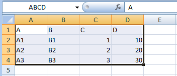
The following command loads this data to initialize parameter D and index Z:

load ABCD.xls range=ABCD : Z=[A,B,C] Y=D ;

Thus, the syntax for loading data from spreadsheets only differs from CSV and ASCII text files by the use of the range option.

When loading from a relational database, the data source specification is a filename or data connection string. Access to a database may be restricted, and thus the specification of username and password options may be required. Alternatively, these options can be specified within a data connection string.

A variety of database interface packages are available within Python. The using option is used to specify the database interface package that will be used to access a database. For example, the pyodbc interface can be used to connect to Excel spreadsheets. The following command loads data from the Excel spreadsheet ABCD.xls using the pyodbc interface. The command loads this data to initialize parameter D and index Z:

load ABCD.xls using=pyodbc table=ABCD : Z=[A,B,C] Y=D ;

The using option specifies that the pyodbc package will be used to connect with the Excel spreadsheet. The table option specifies that the table ABCD is loaded from this spreadsheet. Similarly, the following command specifies a data connection string to specify the ODBC driver explicitly:

load "Driver={Microsoft Excel Driver (*.xls)}; Dbq=ABCD.xls;" 
    using=pyodbc 
    table=ABCD : Z=[A,B,C] Y=D ;

ODBC drivers are generally tailored to the type of data source that they work with; this syntax illustrates how the load command can be tailored to the details of the database that a user is working with.

The previous examples specified the table option, which declares the name of a relational table in a database. Many databases support the Structured Query Language (SQL), which can be used to dynamically compose a relational table from other tables in a database. The classic diet problem will be used to illustrate the use of SQL queries to initialize a Pyomo model. In this problem, a customer is faced with the task of minimizing the cost for a meal at a fast food restaurant – they must purchase a sandwich, side, and a drink for the lowest cost. The following is a Pyomo model for this problem:

#  ___________________________________________________________________________
#
#  Pyomo: Python Optimization Modeling Objects
#  Copyright (c) 2008-2024
#  National Technology and Engineering Solutions of Sandia, LLC
#  Under the terms of Contract DE-NA0003525 with National Technology and
#  Engineering Solutions of Sandia, LLC, the U.S. Government retains certain
#  rights in this software.
#  This software is distributed under the 3-clause BSD License.
#  ___________________________________________________________________________

# diet1.py
from pyomo.environ import *

infinity = float('inf')
MAX_FOOD_SUPPLY = 20.0  # There is a finite food supply

model = AbstractModel()

# --------------------------------------------------------

model.FOOD = Set()
model.cost = Param(model.FOOD, within=PositiveReals)
model.f_min = Param(model.FOOD, within=NonNegativeReals, default=0.0)


def f_max_validate(model, value, j):
    return model.f_max[j] > model.f_min[j]


model.f_max = Param(model.FOOD, validate=f_max_validate, default=MAX_FOOD_SUPPLY)

model.NUTR = Set()
model.n_min = Param(model.NUTR, within=NonNegativeReals, default=0.0)
model.n_max = Param(model.NUTR, default=infinity)
model.amt = Param(model.NUTR, model.FOOD, within=NonNegativeReals)

# --------------------------------------------------------


def Buy_bounds(model, i):
    return (model.f_min[i], model.f_max[i])


model.Buy = Var(model.FOOD, bounds=Buy_bounds, within=NonNegativeIntegers)

# --------------------------------------------------------


def Total_Cost_rule(model):
    return sum(model.cost[j] * model.Buy[j] for j in model.FOOD)


model.Total_Cost = Objective(rule=Total_Cost_rule, sense=minimize)

# --------------------------------------------------------


def Entree_rule(model):
    entrees = [
        'Cheeseburger',
        'Ham Sandwich',
        'Hamburger',
        'Fish Sandwich',
        'Chicken Sandwich',
    ]
    return sum(model.Buy[e] for e in entrees) >= 1


model.Entree = Constraint(rule=Entree_rule)


def Side_rule(model):
    sides = ['Fries', 'Sausage Biscuit']
    return sum(model.Buy[s] for s in sides) >= 1


model.Side = Constraint(rule=Side_rule)


def Drink_rule(model):
    drinks = ['Lowfat Milk', 'Orange Juice']
    return sum(model.Buy[d] for d in drinks) >= 1


model.Drink = Constraint(rule=Drink_rule)

Suppose that the file diet1.sqlite be a SQLite database file that contains the following data in the Food table:

FOOD	cost
Cheeseburger	1.84
Ham Sandwich	2.19
Hamburger	1.84
Fish Sandwich	1.44
Chicken Sandwich	2.29
Fries	0.77
Sausage Biscuit	1.29
Lowfat Milk	0.60
Orange Juice	0.72

In addition, the Food table has two additional columns, f_min and f_max, with no data for any row. These columns exist to match the structure for the parameters used in the model.

We can solve the diet1 model using the Python definition in diet1.py and the data from this database. The file diet.sqlite.dat specifies a load command that uses that sqlite3 data manager and embeds a SQL query to retrieve the data:

# File diet.sqlite.dat

load "diet.sqlite" 
     using=sqlite3 
     query="SELECT FOOD,cost,f_min,f_max FROM Food" 
     : FOOD=[FOOD] cost f_min f_max ;

The PyODBC driver module will pass the SQL query through an Access ODBC connector, extract the data from the diet1.mdb file, and return it to Pyomo. The Pyomo ODBC handler can then convert the data received into the proper format for solving the model internally. More complex SQL queries are possible, depending on the underlying database and ODBC driver in use. However, the name and ordering of the columns queried are specified in the Pyomo data file; using SQL wildcards (e.g., SELECT *) or column aliasing (e.g., SELECT f AS FOOD) may cause errors in Pyomo’s mapping of relational data to parameters.

The include Command

The include command allows a data command file to execute data commands from another file. For example, the following command file executes data commands from ex1.dat and then ex2.dat:

include ex1.dat;
include ex2.dat;

Pyomo is sensitive to the order of execution of data commands, since data commands can redefine set and parameter values. The include command respects this data ordering; all data commands in the included file are executed before the remaining data commands in the current file are executed.

The namespace Keyword

The namespace keyword is not a data command, but instead it is used to structure the specification of Pyomo’s data commands. Specifically, a namespace declaration is used to group data commands and to provide a group label. Consider the following data command file:

set C := 1 2 3 ;

namespace ns1
{
    set C := 4 5 6 ;
}

namespace ns2
{
    set C := 7 8 9 ;
}

This data file defines two namespaces: ns1 and ns2 that initialize a set C. By default, data commands contained within a namespace are ignored during model construction; when no namespaces are specified, the set C has values 1,2,3. When namespace ns1 is specified, then the set C values are overridden with the set 4,5,6.

Data Portals

Pyomo’s DataPortal class standardizes the process of constructing model instances by managing the process of loading data from different data sources in a uniform manner. A DataPortal object can load data from the following data sources:

• TAB File: A text file format that uses whitespace to separate columns of values in each row of a table.

• CSV File: A text file format that uses comma or other delimiters to separate columns of values in each row of a table.

• JSON File: A popular lightweight data-interchange format that is easily parsed.

• YAML File: A human friendly data serialization standard.

• XML File: An extensible markup language for documents and data structures. XML files can represent tabular data.

• Excel File: A spreadsheet data format that is primarily used by the Microsoft Excel application.

• Database: A relational database.

• DAT File: A Pyomo data command file.

Note that most of these data formats can express tabular data.

Warning

The DataPortal class requires the installation of Python packages to support some of these data formats:

• YAML File: pyyaml

• Excel File: win32com, openpyxl or xlrd

  These packages support different data Excel data formats: the win32com package supports .xls, .xlsm and .xlsx, the openpyxl package supports .xlsx and the xlrd package supports .xls.

• Database: pyodbc, pypyodbc, sqlite3 or pymysql

  These packages support different database interface APIs: the pyodbc and pypyodbc packages support the ODBC database API, the sqlite3 package uses the SQLite C library to directly interface with databases using the DB-API 2.0 specification, and pymysql is a pure-Python MySQL client.

DataPortal objects can be used to initialize both concrete and abstract Pyomo models. Consider the file A.tab, which defines a simple set with a tabular format:

A
A1
A2
A3

The load method is used to load data into a DataPortal object. Components in a concrete model can be explicitly initialized with data loaded by a DataPortal object:

data = DataPortal()
data.load(filename='A.tab', set="A", format="set")

model = ConcreteModel()
model.A = Set(initialize=data['A'])

All data needed to initialize an abstract model must be provided by a DataPortal object, and the use of the DataPortal object to initialize components is automated for the user:

model = AbstractModel()
model.A = Set()
data = DataPortal()
data.load(filename='A.tab', set=model.A)
instance = model.create_instance(data)

Note the difference in the execution of the load method in these two examples: for concrete models data is loaded by name and the format must be specified, and for abstract models the data is loaded by component, from which the data format can often be inferred.

The load method opens the data file, processes it, and loads the data in a format that can be used to construct a model instance. The load method can be called multiple times to load data for different sets or parameters, or to override data processed earlier. The load method takes a variety of arguments that define how data is loaded:

• filename: This option specifies the source data file.

• format: This option specifies the how to interpret data within a table. Valid formats are: set, set_array, param, table, array, and transposed_array.

• set: This option is either a string or model compent that defines a set that will be initialized with this data.

• param: This option is either a string or model compent that defines a parameter that will be initialized with this data. A list or tuple of strings or model components can be used to define multiple parameters that are initialized.

• index: This option is either a string or model compent that defines an index set that will be initialized with this data.

• using: This option specifies the Python package used to load this data source. This option is used when loading data from databases.

• select: This option defines the columns that are selected from the data source. The column order may be changed from the data source, which allows the DataPortal object to define

• namespace: This option defines the data namespace that will contain this data.

The use of these options is illustrated below.

The DataPortal class also provides a simple API for accessing set and parameter data that are loaded from different data sources. The [] operator is used to access set and parameter values. Consider the following example, which loads data and prints the value of the [] operator:

data = DataPortal()
data.load(filename='A.tab', set="A", format="set")
print(data['A'])  # ['A1', 'A2', 'A3']

data.load(filename='Z.tab', param="z", format="param")
print(data['z'])  # 1.1

data.load(filename='Y.tab', param="y", format="table")
for key in sorted(data['y']):
    print("%s %s" % (key, data['y'][key]))

The DataPortal class also has several methods for iterating over the data that has been loaded:

• keys(): Returns an iterator of the data keys.

• values(): Returns an iterator of the data values.

• items(): Returns an iterator of (name, value) tuples from the data.

Finally, the data() method provides a generic mechanism for accessing the underlying data representation used by DataPortal objects.

Loading Structured Data

JSON and YAML files are structured data formats that are well-suited for data serialization. These data formats do not represent data in tabular format, but instead they directly represent set and parameter values with lists and dictionaries:

• Simple Set: a list of string or numeric value

• Indexed Set: a dictionary that maps an index to a list of string or numeric value

• Simple Parameter: a string or numeric value

• Indexed Parameter: a dictionary that maps an index to a numeric value

For example, consider the following JSON file:

{   "A": ["A1", "A2", "A3"],
    "B": [[1, "B1"], [2, "B2"], [3, "B3"]],
    "C": {"A1": [1, 2, 3], "A3": [10, 20, 30]},
    "p": 0.1,
    "q": {"A1": 3.3, "A2": 3.4, "A3": 3.5},
    "r": [   {"index": [1, "B1"], "value": 3.3},
             {"index": [2, "B2"], "value": 3.4},
             {"index": [3, "B3"], "value": 3.5}]}

The data in this file can be used to load the following model:

model = AbstractModel()
data = DataPortal()
model.A = Set()
model.B = Set(dimen=2)
model.C = Set(model.A)
model.p = Param()
model.q = Param(model.A)
model.r = Param(model.B)
data.load(filename='T.json')

Note that no set or param option needs to be specified when loading a JSON or YAML file. All of the set and parameter data in the file are loaded by the DataPortal> object, and only the data needed for model construction is used.

The following YAML file has a similar structure:

A: [A1, A2, A3]
B:
- [1, B1]
- [2, B2]
- [3, B3]
C:
  'A1': [1, 2, 3]
  'A3': [10, 20, 30]
p: 0.1
q: {A1: 3.3, A2: 3.4, A3: 3.5}
r:
- index: [1, B1]
  value: 3.3
- index: [2, B2]
  value: 3.4
- index: [3, B3]
  value: 3.5

The data in this file can be used to load a Pyomo model with the same syntax as a JSON file:

model = AbstractModel()
data = DataPortal()
model.A = Set()
model.B = Set(dimen=2)
model.C = Set(model.A)
model.p = Param()
model.q = Param(model.A)
model.r = Param(model.B)
data.load(filename='T.yaml')

Loading Tabular Data

Many data sources supported by Pyomo are tabular data formats. Tabular data is numerical or textual data that is organized into one or more simple tables, where data is arranged in a matrix. Each table consists of a matrix of numeric string values, simple strings, and quoted strings. All rows have the same length, all columns have the same length, and the first row typically represents labels for the column data.

The following section describes the tabular data sources supported by Pyomo, and the subsequent sections illustrate ways that data can be loaded from tabular data using TAB files. Subsequent sections describe options for loading data from Excel spreadsheets and relational databases.

Tabular Data

TAB files represent tabular data in an ascii file using whitespace as a delimiter. A TAB file consists of rows of values, where each row has the same length. For example, the file PP.tab has the format:

A  B  PP
A1 B1 4.3
A2 B2 4.4
A3 B3 4.5

CSV files represent tabular data in a format that is very similar to TAB files. Pyomo assumes that a CSV file consists of rows of values, where each row has the same length. For example, the file PP.csv has the format:

A,B,PP
A1,B1,4.3
A2,B2,4.4
A3,B3,4.5

Excel spreadsheets can express complex data relationships. A range is a contiguous, rectangular block of cells in an Excel spreadsheet. Thus, a range in a spreadsheet has the same tabular structure as is a TAB file or a CSV file. For example, consider the file excel.xls that has the range PPtable:

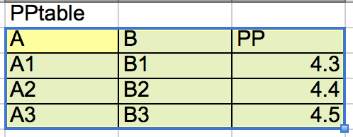
A relational database is an application that organizes data into one or more tables (or relations) with a unique key in each row. Tables both reflect the data in a database as well as the result of queries within a database.

XML files represent tabular using table and row elements. Each sub-element of a row element represents a different column, where each row has the same length. For example, the file PP.xml has the format:

<table>
  <row>
    <A value="A1"/><B value="B1"/><PP value="4.3"/>
  </row>
  <row>
    <A value="A2"/><B value="B2"/><PP value="4.4"/>
  </row>
  <row>
    <A value="A3"/><B value="B3"/><PP value="4.5"/>
  </row>
</table>

Loading Set Data

The set option is used specify a Set component that is loaded with data.

Loading a Simple Set

Consider the file A.tab, which defines a simple set:

A
A1
A2
A3

In the following example, a DataPortal object loads data for a simple set A:

model = AbstractModel()
model.A = Set()
data = DataPortal()
data.load(filename='A.tab', set=model.A)
instance = model.create_instance(data)

Loading a Set of Tuples

Consider the file C.tab:

A  B
A1 1
A1 2
A1 3
A2 1
A2 2
A2 3
A3 1
A3 2
A3 3

In the following example, a DataPortal object loads data for a two-dimensional set C:

model = AbstractModel()
model.C = Set(dimen=2)
data = DataPortal()
data.load(filename='C.tab', set=model.C)
instance = model.create_instance(data)

In this example, the column titles do not directly impact the process of loading data. Column titles can be used to select a subset of columns from a table that is loaded (see below).

Loading a Set Array

Consider the file D.tab, which defines an array representation of a two-dimensional set:

B  A1  A2  A3
1  +   -   -
2  -   +   -
3  -   -   +

In the following example, a DataPortal object loads data for a two-dimensional set D:

model = AbstractModel()
model.D = Set(dimen=2)
data = DataPortal()
data.load(filename='D.tab', set=model.D, format='set_array')
instance = model.create_instance(data)

The format option indicates that the set data is declared in a array format.

Loading Parameter Data

The param option is used specify a Param component that is loaded with data.

Loading a Simple Parameter

The simplest parameter is simply a singleton value. Consider the file Z.tab:

1.1

In the following example, a DataPortal object loads data for a simple parameter z:

model = AbstractModel()
data = DataPortal()
model.z = Param()
data.load(filename='Z.tab', param=model.z)
instance = model.create_instance(data)

Loading an Indexed Parameter

An indexed parameter can be defined by a single column in a table. For example, consider the file Y.tab:

A  Y
A1 3.3
A2 3.4
A3 3.5

In the following example, a DataPortal object loads data for an indexed parameter y:

model = AbstractModel()
data = DataPortal()
model.A = Set(initialize=['A1', 'A2', 'A3'])
model.y = Param(model.A)
data.load(filename='Y.tab', param=model.y)
instance = model.create_instance(data)

When column names are not used to specify the index and parameter data, then the DataPortal object assumes that the rightmost column defines parameter values. In this file, the A column contains the index values, and the Y column contains the parameter values.

Loading Set and Parameter Values

Note that the data for set A is predefined in the previous example. The index set can be loaded with the parameter data using the index option. In the following example, a DataPortal object loads data for set A and the indexed parameter y

model = AbstractModel()
data = DataPortal()
model.A = Set()
model.y = Param(model.A)
data.load(filename='Y.tab', param=model.y, index=model.A)
instance = model.create_instance(data)

An index set with multiple dimensions can also be loaded with an indexed parameter. Consider the file PP.tab:

A  B  PP
A1 B1 4.3
A2 B2 4.4
A3 B3 4.5

In the following example, a DataPortal object loads data for a tuple set and an indexed parameter:

model = AbstractModel()
data = DataPortal()
model.A = Set(dimen=2)
model.p = Param(model.A)
data.load(filename='PP.tab', param=model.p, index=model.A)
instance = model.create_instance(data)

Loading a Parameter with Missing Values

Missing parameter data can be expressed in two ways. First, parameter data can be defined with indices that are a subset of valid indices in the model. The following example loads the indexed parameter y:

model = AbstractModel()
data = DataPortal()
model.A = Set(initialize=['A1', 'A2', 'A3', 'A4'])
model.y = Param(model.A)
data.load(filename='Y.tab', param=model.y)
instance = model.create_instance(data)

The model defines an index set with four values, but only three parameter values are declared in the data file Y.tab.

Parameter data can also be declared with missing values using the period (.) symbol. For example, consider the file S.tab:

A  B  PP
A1 B1 4.3
A2 B2 4.4
A3 B3 4.5

In the following example, a DataPortal object loads data for the index set A and indexed parameter y:

model = AbstractModel()
data = DataPortal()
model.A = Set()
model.s = Param(model.A)
data.load(filename='S.tab', param=model.s, index=model.A)
instance = model.create_instance(data)

The period (.) symbol indicates a missing parameter value, but the index set A contains the index value for the missing parameter.

Loading Multiple Parameters

Multiple parameters can be initialized at once by specifying a list (or tuple) of component parameters. Consider the file XW.tab:

A  X   W
A1 3.3 4.3
A2 3.4 4.4
A3 3.5 4.5

In the following example, a DataPortal object loads data for parameters x and w:

model = AbstractModel()
data = DataPortal()
model.A = Set(initialize=['A1', 'A2', 'A3'])
model.x = Param(model.A)
model.w = Param(model.A)
data.load(filename='XW.tab', param=(model.x, model.w))
instance = model.create_instance(data)

Selecting Parameter Columns

We have previously noted that the column names do not need to be specified to load set and parameter data. However, the select option can be to identify the columns in the table that are used to load parameter data. This option specifies a list (or tuple) of column names that are used, in that order, to form the table that defines the component data.

For example, consider the following load declaration:

model = AbstractModel()
data = DataPortal()
model.A = Set()
model.w = Param(model.A)
data.load(filename='XW.tab', select=('A', 'W'), param=model.w, index=model.A)
instance = model.create_instance(data)

The columns A and W are selected from the file XW.tab, and a single parameter is defined.

Loading a Parameter Array

Consider the file U.tab, which defines an array representation of a multiply-indexed parameter:

I  A1  A2  A3
I1 1.3 2.3 3.3
I2 1.4 2.4 3.4
I3 1.5 2.5 3.5
I4 1.6 2.6 3.6

In the following example, a DataPortal object loads data for a two-dimensional parameter u:

model = AbstractModel()
data = DataPortal()
model.A = Set(initialize=['A1', 'A2', 'A3'])
model.I = Set(initialize=['I1', 'I2', 'I3', 'I4'])
model.u = Param(model.I, model.A)
data.load(filename='U.tab', param=model.u, format='array')
instance = model.create_instance(data)

The format option indicates that the parameter data is declared in a array format. The format option can also indicate that the parameter data should be transposed.

model = AbstractModel()
data = DataPortal()
model.A = Set(initialize=['A1', 'A2', 'A3'])
model.I = Set(initialize=['I1', 'I2', 'I3', 'I4'])
model.t = Param(model.A, model.I)
data.load(filename='U.tab', param=model.t, format='transposed_array')
instance = model.create_instance(data)

Note that the transposed parameter data changes the index set for the parameter.

Loading from Spreadsheets and Databases

Tabular data can be loaded from spreadsheets and databases using auxiliary Python packages that provide an interface to these data formats. Data can be loaded from Excel spreadsheets using the win32com, xlrd and openpyxl packages. For example, consider the following range of cells, which is named PPtable:

In the following example, a DataPortal object loads the named range PPtable from the file excel.xls:

model = AbstractModel()
data = DataPortal()
model.A = Set(dimen=2)
model.p = Param(model.A)
data.load(filename='excel.xls', range='PPtable', param=model.p, index=model.A)
instance = model.create_instance(data)

Note that the range option is required to specify the table of cell data that is loaded from the spreadsheet.

There are a variety of ways that data can be loaded from a relational database. In the simplest case, a table can be specified within a database:

model = AbstractModel()
data = DataPortal()
model.A = Set(dimen=2)
model.p = Param(model.A)
data.load(
    filename='PP.sqlite', using='sqlite3', table='PPtable', param=model.p, index=model.A
)
instance = model.create_instance(data)

In this example, the interface sqlite3 is used to load data from an SQLite database in the file PP.sqlite. More generally, an SQL query can be specified to dynamically generate a table. For example:

model = AbstractModel()
data = DataPortal()
model.A = Set()
model.p = Param(model.A)
data.load(
    filename='PP.sqlite',
    using='sqlite3',
    query="SELECT A,PP FROM PPtable",
    param=model.p,
    index=model.A,
)
instance = model.create_instance(data)

Data Namespaces

The DataPortal class supports the concept of a namespace to organize data into named groups that can be enabled or disabled during model construction. Various DataPortal methods have an optional namespace argument that defaults to None:

• data(name=None, namespace=None): Returns the data associated with data in the specified namespace

• []: For a DataPortal object data, the function data['A'] returns data corresponding to A in the default namespace, and data['ns1','A'] returns data corresponding to A in namespace ns1.

• namespaces(): Returns an iteratore for the data namespaces.

• keys(namespace=None): Returns an iterator of the data keys in the specified namespace.

• values(namespace=None): Returns and iterator of the data values in the specified namespace.

• items(namespace=None): Returns an iterator of (name, value) tuples in the specified namespace.

By default, data within a namespace are ignored during model construction. However, concrete models can be initialized with data from a specific namespace. Further, abstract models can be initialized with a list of namespaces that define the data used to initialized model components. For example, the following script generates two model instances from an abstract model using data loaded into different namespaces:

model = AbstractModel()
model.C = Set(dimen=2)
data = DataPortal()
data.load(filename='C.tab', set=model.C, namespace='ns1')
data.load(filename='D.tab', set=model.C, namespace='ns2', format='set_array')
instance1 = model.create_instance(data, namespaces=['ns1'])
instance2 = model.create_instance(data, namespaces=['ns2'])

Storing Data from Pyomo Models

Currently, Pyomo has rather limited capabilities for storing model data into standard Python data types and serialized data formats. However, this capability is under active development.

Storing Model Data in Excel

TODO

More here.

The pyomo Command

The pyomo command is issued to the DOS prompt or a Unix shell. To see a list of Pyomo command line options, use:

pyomo solve --help

Note

There are two dashes before help.

In this section we will detail some of the options.

Passing Options to a Solver

To pass arguments to a solver when using the pyomo solve command, append the Pyomo command line with the argument --solver-options= followed by an argument that is a string to be sent to the solver (perhaps with dashes added by Pyomo). So for most MIP solvers, the mip gap can be set using

--solver-options="mipgap=0.01"

Multiple options are separated by a space. Options that do not take an argument should be specified with the equals sign followed by either a space or the end of the string.

For example, to specify that the solver is GLPK, then to specify a mipgap of two percent and the GLPK cuts option, use

--solver=glpk --solver-options="mipgap=0.02 cuts="

If there are multiple “levels” to the keyword, as is the case for some Gurobi and CPLEX options, the tokens are separated by underscore. For example, mip cuts all would be specified as mip_cuts_all. For another example, to set the solver to be CPLEX, then to set a mip gap of one percent and to specify ‘y’ for the sub-option numerical to the option emphasis use

--solver=cplex --solver-options="mipgap=0.001 emphasis_numerical=y"

See Sending Options to the Solver for a discussion of passing options in a script.

Troubleshooting

Many of things that can go wrong are covered by error messages, but sometimes they can be confusing or do not provide enough information. Depending on what the troubles are, there might be ways to get a little additional information.

If there are syntax errors in the model file, for example, it can occasionally be helpful to get error messages directly from the Python interpreter rather than through Pyomo. Suppose the name of the model file is scuc.py, then

python scuc.py

can sometimes give useful information for fixing syntax errors.

When there are no syntax errors, but there troubles reading the data or generating the information to pass to a solver, then the --verbose option provides a trace of the execution of Pyomo. The user should be aware that for some models this option can generate a lot of output.

If there are troubles with solver (i.e., after Pyomo has output “Applying Solver”), it is often helpful to use the option --stream-solver that causes the solver output to be displayed rather than trapped. (See <<TeeTrue>> for information about getting this output in a script). Advanced users may wish to examine the files that are generated to be passed to a solver. The type of file generated is controlled by the --solver-io option and the --keepfiles option instructs pyomo to keep the files and output their names. However, the --symbolic-solver-labels option should usually also be specified so that meaningful names are used in these files.

When there seem to be troubles expressing the model, it is often useful to embed print commands in the model in places that will yield helpful information. Consider the following snippet:

def ax_constraint_rule(model, i):
    # return the expression for the constraint for i
    print("ax_constraint_rule was called for i=", str(i))
    return sum(model.a[i, j] * model.x[j] for j in model.J) >= model.b[i]


# the next line creates one constraint for each member of the set model.I
model.AxbConstraint = Constraint(model.I, rule=ax_constraint_rule)

The effect will be to output every member of the set model.I at the time the constraint named model.AxbConstraint is constructed.

Direct Interfaces to Solvers

In many applications, the default solver interface works well. However, in some cases it is useful to specify the interface using the solver-io option. For example, if the solver supports a direct Python interface, then the option would be specified on the command line as

--solver-io=python

Here are some of the choices:

• lp: generate a standard linear programming format file with filename extension lp

• nlp: generate a file with a standard format that supports linear and nonlinear optimization with filename extension n1lp

• os: generate an OSiL format XML file.

• python: use the direct Python interface.

Note

Not all solvers support all interfaces.

BuildAction and BuildCheck

This is a somewhat advanced topic. In some cases, it is desirable to trigger actions to be done as part of the model building process. The BuildAction function provides this capability in a Pyomo model. It takes as arguments optional index sets and a function to perform the action. For example,

model.BuildBpts = BuildAction(model.J, rule=bpts_build)

calls the function bpts_build for each member of model.J. The function bpts_build should have the model and a variable for the members of model.J as formal arguments. In this example, the following would be a valid declaration for the function:

def bpts_build(model, j):

A full example, which extends the Symbolic Index Sets and Piecewise Linear Expressions examples, is

#  ___________________________________________________________________________
#
#  Pyomo: Python Optimization Modeling Objects
#  Copyright (c) 2008-2024
#  National Technology and Engineering Solutions of Sandia, LLC
#  Under the terms of Contract DE-NA0003525 with National Technology and
#  Engineering Solutions of Sandia, LLC, the U.S. Government retains certain
#  rights in this software.
#  This software is distributed under the 3-clause BSD License.
#  ___________________________________________________________________________

# abstract2piecebuild.py
# Similar to abstract2piece.py, but the breakpoints are created using a build action

from pyomo.environ import *

model = AbstractModel()

model.I = Set()
model.J = Set()

model.a = Param(model.I, model.J)
model.b = Param(model.I)
model.c = Param(model.J)

model.Topx = Param(default=6.1)  # range of x variables
model.PieceCnt = Param(default=100)

# the next line declares a variable indexed by the set J
model.x = Var(model.J, domain=NonNegativeReals, bounds=(0, model.Topx))
model.y = Var(model.J, domain=NonNegativeReals)

# to avoid warnings, we set breakpoints beyond the bounds
# we are using a dictionary so that we can have different
# breakpoints for each index. But we won't.
model.bpts = {}


def bpts_build(model, j):
    model.bpts[j] = []
    for i in range(model.PieceCnt + 2):
        model.bpts[j].append(float((i * model.Topx) / model.PieceCnt))


# The object model.BuildBpts is not referred to again;
# the only goal is to trigger the action at build time
model.BuildBpts = BuildAction(model.J, rule=bpts_build)


def f4(model, j, xp):
    # we not need j in this example, but it is passed as the index for the constraint
    return xp**4


model.ComputePieces = Piecewise(
    model.J, model.y, model.x, pw_pts=model.bpts, pw_constr_type='EQ', f_rule=f4
)


def obj_expression(model):
    return summation(model.c, model.y)


model.OBJ = Objective(rule=obj_expression)


def ax_constraint_rule(model, i):
    # return the expression for the constraint for i
    return sum(model.a[i, j] * model.x[j] for j in model.J) >= model.b[i]


# the next line creates one constraint for each member of the set model.I
model.AxbConstraint = Constraint(model.I, rule=ax_constraint_rule)

This example uses the build action to create a model component with breakpoints for a Piecewise Linear Expressions function. The BuildAction is triggered by the assignment to model.BuildBpts. This object is not referenced again, the only goal is to cause the execution of bpts_build, which places data in the model.bpts dictionary. Note that if model.bpts had been a Set, then it could have been created with an initialize argument to the Set declaration. Since it is a special-purpose dictionary to support the Piecewise Linear Expressions functionality in Pyomo, we use a BuildAction.

Another application of BuildAction can be initialization of Pyomo model data from Python data structures, or efficient initialization of Pyomo model data from other Pyomo model data. Consider the Sparse Index Sets example. Rather than using an initialization for each list of sets NodesIn and NodesOut separately using initialize, it is a little more efficient and probably a little clearer, to use a build action.

The full model is:

#  ___________________________________________________________________________
#
#  Pyomo: Python Optimization Modeling Objects
#  Copyright (c) 2008-2024
#  National Technology and Engineering Solutions of Sandia, LLC
#  Under the terms of Contract DE-NA0003525 with National Technology and
#  Engineering Solutions of Sandia, LLC, the U.S. Government retains certain
#  rights in this software.
#  This software is distributed under the 3-clause BSD License.
#  ___________________________________________________________________________

# Isinglebuild.py
# NodesIn and NodesOut are created by a build action using the Arcs
from pyomo.environ import *

model = AbstractModel()

model.Nodes = Set()
model.Arcs = Set(dimen=2)

model.NodesOut = Set(model.Nodes, within=model.Nodes, initialize=[])
model.NodesIn = Set(model.Nodes, within=model.Nodes, initialize=[])


def Populate_In_and_Out(model):
    # loop over the arcs and put the end points in the appropriate places
    for i, j in model.Arcs:
        model.NodesIn[j].add(i)
        model.NodesOut[i].add(j)


model.In_n_Out = BuildAction(rule=Populate_In_and_Out)

model.Flow = Var(model.Arcs, domain=NonNegativeReals)
model.FlowCost = Param(model.Arcs)

model.Demand = Param(model.Nodes)
model.Supply = Param(model.Nodes)


def Obj_rule(model):
    return summation(model.FlowCost, model.Flow)


model.Obj = Objective(rule=Obj_rule, sense=minimize)


def FlowBalance_rule(model, node):
    return (
        model.Supply[node]
        + sum(model.Flow[i, node] for i in model.NodesIn[node])
        - model.Demand[node]
        - sum(model.Flow[node, j] for j in model.NodesOut[node])
        == 0
    )


model.FlowBalance = Constraint(model.Nodes, rule=FlowBalance_rule)

for this model, the same data file can be used as for Isinglecomm.py in Sparse Index Sets such as the toy data file:

set Nodes := CityA CityB CityC ;

set Arcs :=
CityA CityB
CityA CityC
CityC CityB
;

param : FlowCost :=
CityA CityB 1.4
CityA CityC 2.7
CityC CityB 1.6
 ;

param Demand :=
CityA 0
CityB 1
CityC 1
;

param Supply :=
CityA 2
CityB 0
CityC 0
;

Build actions can also be a way to implement data validation, particularly when multiple Sets or Parameters must be analyzed. However, the the BuildCheck component is preferred for this purpose. It executes its rule just like a BuildAction but will terminate the construction of the model instance if the rule returns False.

Model Transformations

Model Scaling Transformation

Good scaling of models can greatly improve the numerical properties of a problem and thus increase reliability and convergence. The core.scale_model transformation allows users to separate scaling of a model from the declaration of the model variables and constraints which allows for models to be written in more natural forms and to be scaled and rescaled as required without having to rewrite the model code.

class pyomo.core.plugins.transform.scaling.ScaleModel(**kwds)

Transformation to scale a model.

This plugin performs variable, constraint, and objective scaling on a model based on the scaling factors in the suffix ‘scaling_factor’ set for the variables, constraints, and/or objective. This is typically done to scale the problem for improved numerical properties.

Supported transformation methods:

• apply_to

• create_using

• propagate_solution

By default, scaling components are renamed with the prefix scaled_. To disable this behavior and scale variables in-place (or keep the same names in a new model), use the rename=False argument to apply_to or create_using.

Examples

>>> from pyomo.environ import *
>>> # create the model
>>> model = ConcreteModel()
>>> model.x = Var(bounds=(-5, 5), initialize=1.0)
>>> model.y = Var(bounds=(0, 1), initialize=1.0)
>>> model.obj = Objective(expr=1e8*model.x + 1e6*model.y)
>>> model.con = Constraint(expr=model.x + model.y == 1.0)
>>> # create the scaling factors
>>> model.scaling_factor = Suffix(direction=Suffix.EXPORT)
>>> model.scaling_factor[model.obj] = 1e-6 # scale the objective
>>> model.scaling_factor[model.con] = 2.0  # scale the constraint
>>> model.scaling_factor[model.x] = 0.2    # scale the x variable
>>> # transform the model
>>> scaled_model = TransformationFactory('core.scale_model').create_using(model)
>>> # print the value of the objective function to show scaling has occurred
>>> print(value(model.x))
1.0
>>> print(value(scaled_model.scaled_x))
0.2
>>> print(value(scaled_model.scaled_x.lb))
-1.0
>>> print(value(model.obj))
101000000.0
>>> print(value(scaled_model.scaled_obj))
101.0

propagate_solution(scaled_model, original_model)

This method takes the solution in scaled_model and maps it back to the original model.

It will also transform duals and reduced costs if the suffixes ‘dual’ and/or ‘rc’ are present. The scaled_model argument must be a model that was already scaled using this transformation as it expects data from the transformation to perform the back mapping.

Parameters:

• scaled_model (Pyomo Model) – The model that was previously scaled with this transformation

• original_model (Pyomo Model) – The original unscaled source model

Setting Scaling Factors

Scaling factors for components in a model are declared using Suffixes, as shown in the example above. In order to define a scaling factor for a component, a Suffix named scaling_factor must first be created to hold the scaling factor(s). Scaling factor suffixes can be declared at any level of the model hierarchy, but scaling factors declared on the higher-level models or Blocks take precedence over those declared at lower levels.

Scaling suffixes are dict-like where each key is a Pyomo component and the value is the scaling factor to be applied to that component.

In the case of indexed components, scaling factors can either be declared for an individual index or for the indexed component as a whole (with scaling factors for individual indices taking precedence over overall scaling factors).

Note

In the case that a scaling factor is declared for a component on at multiple levels of the hierarchy, the highest level scaling factor will be applied.

Note

It is also possible (but not encouraged) to define a “default” scaling factor to be applied to any component for which a specific scaling factor has not been declared by setting a entry in a Suffix with a key of None. In this case, the default value declared closest to the component to be scaled will be used (i.e., the first default value found when walking up the model hierarchy).

Applying Model Scaling

The core.scale_model transformation provides two approaches for creating a scaled model.

In-Place Scaling

The apply_to(model) method can be used to apply scaling directly to an existing model. When using this method, all the variables, constraints and objectives within the target model are replaced with new scaled components and the appropriate scaling factors applied. The model can then be sent to a solver as usual, however the results will be in terms of the scaled components and must be un-scaled by the user.

Creating a New Scaled Model

Alternatively, the create_using(model) method can be used to create a new, scaled version of the model which can be solved. In this case, a clone of the original model is generated with the variables, constraints and objectives replaced by scaled equivalents. Users can then send the scaled model to a solver after which the propagate_solution method can be used to map the scaled solution back onto the original model for further analysis.

The advantage of this approach is that the original model is maintained separately from the scaled model, which facilitates rescaling and other manipulation of the original model after a solution has been found. The disadvantage of this approach is that cloning the model may result in memory issues when dealing with larger models.

Modeling Extensions

Bilevel Programming

pyomo.bilevel provides extensions supporting modeling of multi-level optimization problems.

Dynamic Optimization with pyomo.DAE

The pyomo.DAE modeling extension [PyomoDAE] allows users to incorporate systems of differential algebraic equations (DAE)s in a Pyomo model. The modeling components in this extension are able to represent ordinary or partial differential equations. The differential equations do not have to be written in a particular format and the components are flexible enough to represent higher-order derivatives or mixed partial derivatives. Pyomo.DAE also includes model transformations which use simultaneous discretization approaches to transform a DAE model into an algebraic model. Finally, pyomo.DAE includes utilities for simulating DAE models and initializing dynamic optimization problems.

Modeling Components

Pyomo.DAE introduces three new modeling components to Pyomo:

pyomo.dae.ContinuousSet	Represents a bounded continuous domain
pyomo.dae.DerivativeVar	Represents derivatives in a model and defines how a Var is differentiated
pyomo.dae.Integral	Represents an integral over a continuous domain

As will be shown later, differential equations can be declared using using these new modeling components along with the standard Pyomo Var and Constraint components.

ContinuousSet

This component is used to define continuous bounded domains (for example ‘spatial’ or ‘time’ domains). It is similar to a Pyomo Set component and can be used to index things like variables and constraints. Any number of ContinuousSets can be used to index a component and components can be indexed by both Sets and ContinuousSets in arbitrary order.

In the current implementation, models with ContinuousSet components may not be solved until every ContinuousSet has been discretized. Minimally, a ContinuousSet must be initialized with two numeric values representing the upper and lower bounds of the continuous domain. A user may also specify additional points in the domain to be used as finite element points in the discretization.

class pyomo.dae.ContinuousSet(*args, **kwds)

Represents a bounded continuous domain

Minimally, this set must contain two numeric values defining the bounds of a continuous range. Discrete points of interest may be added to the continuous set. A continuous set is one dimensional and may only contain numerical values.

Parameters:

• initialize (list) – Default discretization points to be included

• bounds (tuple) – The bounding points for the continuous domain. The bounds will be included as discrete points in the ContinuousSet and will be used to bound the points added to the ContinuousSet through the ‘initialize’ argument, a data file, or the add() method

_changed

This keeps track of whether or not the ContinuousSet was changed during discretization. If the user specifies all of the needed discretization points before the discretization then there is no need to go back through the model and reconstruct things indexed by the ContinuousSet

Type:

boolean

_fe

This is a sorted list of the finite element points in the ContinuousSet. i.e. this list contains all the discrete points in the ContinuousSet that are not collocation points. Points that are both finite element points and collocation points will be included in this list.

Type:

list

_discretization_info

This is a dictionary which contains information on the discretization transformation which has been applied to the ContinuousSet.

Type:

dict

construct(values=None)

Constructs a ContinuousSet component

find_nearest_index(target, tolerance=None)

Returns the index of the nearest point in the ContinuousSet.

If a tolerance is specified, the index will only be returned if the distance between the target and the closest point is less than or equal to that tolerance. If there is a tie for closest point, the index on the left is returned.

Parameters:

• target (float) –

• tolerance (float or None) –

Return type:

float or None

get_changed()

Returns flag indicating if the ContinuousSet was changed during discretization

Returns “True” if additional points were added to the ContinuousSet while applying a discretization scheme

Return type:

boolean

get_discretization_info()

Returns a dict with information on the discretization scheme that has been applied to the ContinuousSet.

Return type:

dict

get_finite_elements()

Returns the finite element points

If the ContinuousSet has been discretizaed using a collocation scheme, this method will return a list of the finite element discretization points but not the collocation points within each finite element. If the ContinuousSet has not been discretized or a finite difference discretization was used, this method returns a list of all the discretization points in the ContinuousSet.

Return type:

list of floats

get_lower_element_boundary(point)

Returns the first finite element point that is less than or equal to ‘point’

Parameters:

point (float) –

Return type:

float

get_upper_element_boundary(point)

Returns the first finite element point that is greater or equal to ‘point’

Parameters:

point (float) –

Return type:

float

set_changed(newvalue)

Sets the _changed flag to ‘newvalue’

Parameters:

newvalue (boolean) –

The following code snippet shows examples of declaring a ContinuousSet component on a concrete Pyomo model:

Required imports
>>> from pyomo.environ import *
>>> from pyomo.dae import *

>>> model = ConcreteModel()

Declaration by providing bounds
>>> model.t = ContinuousSet(bounds=(0,5))

Declaration by initializing with desired discretization points
>>> model.x = ContinuousSet(initialize=[0,1,2,5])

Note

A ContinuousSet may not be constructed unless at least two numeric points are provided to bound the continuous domain.

The following code snippet shows an example of declaring a ContinuousSet component on an abstract Pyomo model using the example data file.

set t := 0 0.5 2.25 3.75 5;

Required imports
>>> from pyomo.environ import *
>>> from pyomo.dae import *

>>> model = AbstractModel()

The ContinuousSet below will be initialized using the points
in the data file when a model instance is created.
>>> model.t = ContinuousSet()

Note

If a separate data file is used to initialize a ContinuousSet, it is done using the ‘set’ command and not ‘continuousset’

Note

Most valid ways to declare and initialize a Set can be used to declare and initialize a ContinuousSet. See the documentation for Set for additional options.

Warning

Be careful using a ContinuousSet as an implicit index in an expression, i.e. sum(m.v[i] for i in m.myContinuousSet). The expression will be generated using the discretization points contained in the ContinuousSet at the time the expression was constructed and will not be updated if additional points are added to the set during discretization.

Note

ContinuousSet components are always ordered (sorted) therefore the first() and last() Set methods can be used to access the lower and upper boundaries of the ContinuousSet respectively

DerivativeVar

class pyomo.dae.DerivativeVar(*args, **kwargs)

Represents derivatives in a model and defines how a Var is differentiated

The DerivativeVar component is used to declare a derivative of a Var. The constructor accepts a single positional argument which is the Var that’s being differentiated. A Var may only be differentiated with respect to a ContinuousSet that it is indexed by. The indexing sets of a DerivativeVar are identical to those of the Var it is differentiating.

Parameters:

• sVar (pyomo.environ.Var) – The variable being differentiated

• wrt (pyomo.dae.ContinuousSet or tuple) – Equivalent to withrespectto keyword argument. The ContinuousSet that the derivative is being taken with respect to. Higher order derivatives are represented by including the ContinuousSet multiple times in the tuple sent to this keyword. i.e. wrt=(m.t, m.t) would be the second order derivative with respect to m.t

get_continuousset_list()

Return the a list of ContinuousSet components the derivative is being taken with respect to.

Return type:

list

get_derivative_expression()

Returns the current discretization expression for this derivative or creates an access function to its Var the first time this method is called. The expression gets built up as the discretization transformations are sequentially applied to each ContinuousSet in the model.

get_state_var()

Return the Var that is being differentiated.

Return type:

Var

is_fully_discretized()

Check to see if all the ContinuousSets this derivative is taken with respect to have been discretized.

Return type:

boolean

set_derivative_expression(expr)

Sets``_expr``, an expression representing the discretization equations linking the DerivativeVar to its state Var

The code snippet below shows examples of declaring DerivativeVar components on a Pyomo model. In each case, the variable being differentiated is supplied as the only positional argument and the type of derivative is specified using the ‘wrt’ (or the more verbose ‘withrespectto’) keyword argument. Any keyword argument that is valid for a Pyomo Var component may also be specified.

Required imports
>>> from pyomo.environ import *
>>> from pyomo.dae import *

>>> model = ConcreteModel()
>>> model.s = Set(initialize=['a','b'])
>>> model.t = ContinuousSet(bounds=(0,5))
>>> model.l = ContinuousSet(bounds=(-10,10))

>>> model.x = Var(model.t)
>>> model.y = Var(model.s,model.t)
>>> model.z = Var(model.t,model.l)

Declare the first derivative of model.x with respect to model.t
>>> model.dxdt = DerivativeVar(model.x, withrespectto=model.t)

Declare the second derivative of model.y with respect to model.t
Note that this DerivativeVar will be indexed by both model.s and model.t
>>> model.dydt2 = DerivativeVar(model.y, wrt=(model.t,model.t))

Declare the partial derivative of model.z with respect to model.l
Note that this DerivativeVar will be indexed by both model.t and model.l
>>> model.dzdl = DerivativeVar(model.z, wrt=(model.l), initialize=0)

Declare the mixed second order partial derivative of model.z with respect
to model.t and model.l and set bounds
>>> model.dz2 = DerivativeVar(model.z, wrt=(model.t, model.l), bounds=(-10, 10))

Note

The ‘initialize’ keyword argument will initialize the value of a derivative and is not the same as specifying an initial condition. Initial or boundary conditions should be specified using a Constraint or ConstraintList or by fixing the value of a Var at a boundary point.

Declaring Differential Equations

A differential equations is declared as a standard Pyomo Constraint and is not required to have any particular form. The following code snippet shows how one might declare an ordinary or partial differential equation.

Required imports
>>> from pyomo.environ import *
>>> from pyomo.dae import *

>>> model = ConcreteModel()
>>> model.s = Set(initialize=['a', 'b'])
>>> model.t = ContinuousSet(bounds=(0, 5))
>>> model.l = ContinuousSet(bounds=(-10, 10))

>>> model.x = Var(model.s, model.t)
>>> model.y = Var(model.t, model.l)
>>> model.dxdt = DerivativeVar(model.x, wrt=model.t)
>>> model.dydt = DerivativeVar(model.y, wrt=model.t)
>>> model.dydl2 = DerivativeVar(model.y, wrt=(model.l, model.l))

An ordinary differential equation
>>> def _ode_rule(m, s, t):
...    if t == 0:
...       return Constraint.Skip
...    return m.dxdt[s, t] == m.x[s, t]**2
>>> model.ode = Constraint(model.s, model.t, rule=_ode_rule)

A partial differential equation
>>> def _pde_rule(m, t, l):
...    if t == 0 or l == m.l.first() or l == m.l.last():
...       return Constraint.Skip
...    return m.dydt[t, l] == m.dydl2[t, l]
>>> model.pde = Constraint(model.t, model.l, rule=_pde_rule)

By default, a Constraint declared over a ContinuousSet will be applied at every discretization point contained in the set. Often a modeler does not want to enforce a differential equation at one or both boundaries of a continuous domain. This may be addressed explicitly in the Constraint declaration using Constraint.Skip as shown above. Alternatively, the desired constraints can be deactivated just before the model is sent to a solver as shown below.

>>> def _ode_rule(m, s, t):
...    return m.dxdt[s, t] == m.x[s, t]**2
>>> model.ode = Constraint(model.s, model.t, rule=_ode_rule)

>>> def _pde_rule(m, t, l):
...    return m.dydt[t, l] == m.dydl2[t, l]
>>> model.pde = Constraint(model.t, model.l, rule=_pde_rule)

Declare other model components and apply a discretization transformation
...

Deactivate the differential equations at certain boundary points
>>> for con in model.ode[:, model.t.first()]:
...    con.deactivate()

>>> for con in model.pde[0, :]:
...    con.deactivate()

>>> for con in model.pde[:, model.l.first()]:
...    con.deactivate()

>>> for con in model.pde[:, model.l.last()]:
...   con.deactivate()

Solve the model
...

Note

If you intend to use the pyomo.DAE Simulator on your model then you must use constraint deactivation instead of constraint skipping in the differential equation rule.

Declaring Integrals

Warning

The Integral component is still under development and considered a prototype. It currently includes only basic functionality for simple integrals. We welcome feedback on the interface and functionality but we do not recommend using it on general models. Instead, integrals should be reformulated as differential equations.

class pyomo.dae.Integral(*args, **kwds)

Represents an integral over a continuous domain

The Integral component can be used to represent an integral taken over the entire domain of a ContinuousSet. Once every ContinuousSet in a model has been discretized, any integrals in the model will be converted to algebraic equations using the trapezoid rule. Future development will include more sophisticated numerical integration methods.

Parameters:

• *args – Every indexing set needed to evaluate the integral expression

• wrt (ContinuousSet) – The continuous domain over which the integral is being taken

• rule (function) – Function returning the expression being integrated

get_continuousset()

Return the ContinuousSet the integral is being taken over

Declaring an Integral component is similar to declaring an Expression component. A simple example is shown below:

>>> model = ConcreteModel()
>>> model.time = ContinuousSet(bounds=(0,10))
>>> model.X = Var(model.time)
>>> model.scale = Param(initialize=1E-3)

>>> def _intX(m,t):
...    return m.X[t]
>>> model.intX = Integral(model.time,wrt=model.time,rule=_intX)

>>> def _obj(m):
...    return m.scale*m.intX
>>> model.obj = Objective(rule=_obj)

Notice that the positional arguments supplied to the Integral declaration must include all indices needed to evaluate the integral expression. The integral expression is defined in a function and supplied to the ‘rule’ keyword argument. Finally, a user must specify a ContinuousSet that the integral is being evaluated over. This is done using the ‘wrt’ keyword argument.

Note

The ContinuousSet specified using the ‘wrt’ keyword argument must be explicitly specified as one of the indexing sets (meaning it must be supplied as a positional argument). This is to ensure consistency in the ordering and dimension of the indexing sets

After an Integral has been declared, it can be used just like a Pyomo Expression component and can be included in constraints or the objective function as shown above.

If an Integral is specified with multiple positional arguments, i.e. multiple indexing sets, the final component will be indexed by all of those sets except for the ContinuousSet that the integral was taken over. In other words, the ContinuousSet specified with the ‘wrt’ keyword argument is removed from the indexing sets of the Integral even though it must be specified as a positional argument. This should become more clear with the following example showing a double integral over the ContinuousSet components model.t1 and model.t2. In addition, the expression is also indexed by the Set model.s. The mathematical representation and implementation in Pyomo are shown below:

\[\sum_{s} \int_{t_2} \int_{t_1} \! X(t_1, t_2, s) \, dt_1 \, dt_2\]

>>> model = ConcreteModel()
>>> model.t1 = ContinuousSet(bounds=(0, 10))
>>> model.t2 = ContinuousSet(bounds=(-1, 1))
>>> model.s = Set(initialize=['A', 'B', 'C'])

>>> model.X = Var(model.t1, model.t2, model.s)

>>> def _intX1(m, t1, t2, s):
...    return m.X[t1, t2, s]
>>> model.intX1 = Integral(model.t1, model.t2, model.s, wrt=model.t1,
...                        rule=_intX1)

>>> def _intX2(m, t2, s):
...    return m.intX1[t2, s]
>>> model.intX2 = Integral(model.t2, model.s, wrt=model.t2, rule=_intX2)

>>> def _obj(m):
...    return sum(m.intX2[k] for k in m.s)
>>> model.obj = Objective(rule=_obj)

Discretization Transformations

Before a Pyomo model with DerivativeVar or Integral components can be sent to a solver it must first be sent through a discretization transformation. These transformations approximate any derivatives or integrals in the model by using a numerical method. The numerical methods currently included in pyomo.DAE discretize the continuous domains in the problem and introduce equality constraints which approximate the derivatives and integrals at the discretization points. Two families of discretization schemes have been implemented in pyomo.DAE, Finite Difference and Collocation. These schemes are described in more detail below.

Note

The schemes described here are for derivatives only. All integrals will be transformed using the trapezoid rule.

The user must write a Python script in order to use these discretizations, they have not been tested on the pyomo command line. Example scripts are shown below for each of the discretization schemes. The transformations are applied to Pyomo model objects which can be further manipulated before being sent to a solver. Examples of this are also shown below.

Finite Difference Transformation

This transformation includes implementations of several finite difference methods. For example, the Backward Difference method (also called Implicit or Backward Euler) has been implemented. The discretization equations for this method are shown below:

\[\begin{split}\begin{array}{l} \mathrm{Given: } \\ \frac{dx}{dt} = f(t, x) , \quad x(t_0) = x_{0} \\ \text{discretize $t$ and $x$ such that } \\ x(t_0 + kh) = x_{k} \\ x_{k + 1} = x_{k} + h * f(t_{k + 1}, x_{k + 1}) \\ t_{k + 1} = t_{k} + h \end{array}\end{split}\]

where \(h\) is the step size between discretization points or the size of each finite element. These equations are generated automatically as Constraints when the backward difference method is applied to a Pyomo model.

There are several discretization options available to a dae.finite_difference transformation which can be specified as keyword arguments to the .apply_to() function of the transformation object. These keywords are summarized below:

Keyword arguments for applying a finite difference transformation:

‘nfe’

The desired number of finite element points to be included in the discretization. The default value is 10.

‘wrt’

Indicates which ContinuousSet the transformation should be applied to. If this keyword argument is not specified then the same scheme will be applied to every ContinuousSet .

‘scheme’

Indicates which finite difference method to apply. Options are ‘BACKWARD’, ‘CENTRAL’, or ‘FORWARD’. The default scheme is the backward difference method.

If the existing number of finite element points in a ContinuousSet is less than the desired number, new discretization points will be added to the set. If a user specifies a number of finite element points which is less than the number of points already included in the ContinuousSet then the transformation will ignore the specified number and proceed with the larger set of points. Discretization points will never be removed from a ContinuousSet during the discretization.

The following code is a Python script applying the backward difference method. The code also shows how to add a constraint to a discretized model.

Discretize model using Backward Difference method
>>> discretizer = TransformationFactory('dae.finite_difference')
>>> discretizer.apply_to(model,nfe=20,wrt=model.time,scheme='BACKWARD')

Add another constraint to discretized model
>>> def _sum_limit(m):
...    return sum(m.x1[i] for i in m.time) <= 50
>>> model.con_sum_limit = Constraint(rule=_sum_limit)

Solve discretized model
>>> solver = SolverFactory('ipopt')
>>> results = solver.solve(model)

Collocation Transformation

This transformation uses orthogonal collocation to discretize the differential equations in the model. Currently, two types of collocation have been implemented. They both use Lagrange polynomials with either Gauss-Radau roots or Gauss-Legendre roots. For more information on orthogonal collocation and the discretization equations associated with this method please see chapter 10 of the book “Nonlinear Programming: Concepts, Algorithms, and Applications to Chemical Processes” by L.T. Biegler.

The discretization options available to a dae.collocation transformation are the same as those described above for the finite difference transformation with different available schemes and the addition of the ‘ncp’ option.

Additional keyword arguments for collocation discretizations:

‘scheme’

The desired collocation scheme, either ‘LAGRANGE-RADAU’ or ‘LAGRANGE-LEGENDRE’. The default is ‘LAGRANGE-RADAU’.

‘ncp’

The number of collocation points within each finite element. The default value is 3.

Note

If the user’s version of Python has access to the package Numpy then any number of collocation points may be specified, otherwise the maximum number is 10.

Note

Any points that exist in a ContinuousSet before discretization will be used as finite element boundaries and not as collocation points. The locations of the collocation points cannot be specified by the user, they must be generated by the transformation.

The following code is a Python script applying collocation with Lagrange polynomials and Radau roots. The code also shows how to add an objective function to a discretized model.

Discretize model using Radau Collocation
>>> discretizer = TransformationFactory('dae.collocation')
>>> discretizer.apply_to(model,nfe=20,ncp=6,scheme='LAGRANGE-RADAU')

Add objective function after model has been discretized
>>> def obj_rule(m):
...    return sum((m.x[i]-m.x_ref)**2 for i in m.time)
>>> model.obj = Objective(rule=obj_rule)

Solve discretized model
>>> solver = SolverFactory('ipopt')
>>> results = solver.solve(model)

Restricting Optimal Control Profiles

When solving an optimal control problem a user may want to restrict the number of degrees of freedom for the control input by forcing, for example, a piecewise constant profile. Pyomo.DAE provides the reduce_collocation_points function to address this use-case. This function is used in conjunction with the dae.collocation discretization transformation to reduce the number of free collocation points within a finite element for a particular variable.

class pyomo.dae.plugins.colloc.Collocation_Discretization_Transformation

reduce_collocation_points(instance, var=None, ncp=None, contset=None)

This method will add additional constraints to a model to reduce the number of free collocation points (degrees of freedom) for a particular variable.

Parameters:

• instance (Pyomo model) – The discretized Pyomo model to add constraints to

• var (pyomo.environ.Var) – The Pyomo variable for which the degrees of freedom will be reduced

• ncp (int) – The new number of free collocation points for var. Must be less that the number of collocation points used in discretizing the model.

• contset (pyomo.dae.ContinuousSet) – The ContinuousSet that was discretized and for which the var will have a reduced number of degrees of freedom

An example of using this function is shown below:

>>> discretizer = TransformationFactory('dae.collocation')
>>> discretizer.apply_to(model, nfe=10, ncp=6)
>>> model = discretizer.reduce_collocation_points(model,
...                                               var=model.u,
...                                               ncp=1,
...                                               contset=model.time)

In the above example, the reduce_collocation_points function restricts the variable model.u to have only 1 free collocation point per finite element, thereby enforcing a piecewise constant profile. Fig. 1 shows the solution profile before and after applying the reduce_collocation_points function.

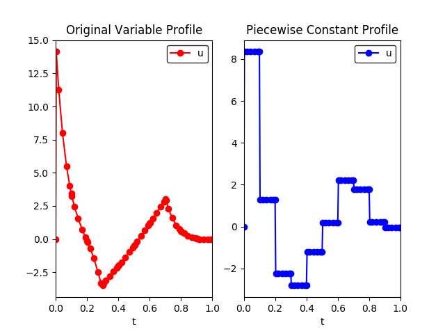
(left) Profile before applying the reduce_collocation_points function (right) Profile after applying the function, restricting model.u to have a piecewise constant profile.

Applying Multiple Discretization Transformations

Discretizations can be applied independently to each ContinuousSet in a model. This allows the user great flexibility in discretizing their model. For example the same numerical method can be applied with different resolutions:

>>> discretizer = TransformationFactory('dae.finite_difference')
>>> discretizer.apply_to(model,wrt=model.t1,nfe=10)
>>> discretizer.apply_to(model,wrt=model.t2,nfe=100)

This also allows the user to combine different methods. For example, applying the forward difference method to one ContinuousSet and the central finite difference method to another ContinuousSet:

>>> discretizer = TransformationFactory('dae.finite_difference')
>>> discretizer.apply_to(model,wrt=model.t1,scheme='FORWARD')
>>> discretizer.apply_to(model,wrt=model.t2,scheme='CENTRAL')

In addition, the user may combine finite difference and collocation discretizations. For example:

>>> disc_fe = TransformationFactory('dae.finite_difference')
>>> disc_fe.apply_to(model,wrt=model.t1,nfe=10)
>>> disc_col = TransformationFactory('dae.collocation')
>>> disc_col.apply_to(model,wrt=model.t2,nfe=10,ncp=5)

If the user would like to apply the same discretization to all ContinuousSet components in a model, just specify the discretization once without the ‘wrt’ keyword argument. This will apply that scheme to all ContinuousSet components in the model that haven’t already been discretized.

Custom Discretization Schemes

A transformation framework along with certain utility functions has been created so that advanced users may easily implement custom discretization schemes other than those listed above. The transformation framework consists of the following steps:

1. Specify Discretization Options

2. Discretize the ContinuousSet(s)

3. Update Model Components

4. Add Discretization Equations

5. Return Discretized Model

If a user would like to create a custom finite difference scheme then they only have to worry about step (4) in the framework. The discretization equations for a particular scheme have been isolated from of the rest of the code for implementing the transformation. The function containing these discretization equations can be found at the top of the source code file for the transformation. For example, below is the function for the forward difference method:

def _forward_transform(v,s):
"""
Applies the Forward Difference formula of order O(h) for first derivatives
"""
    def _fwd_fun(i):
        tmp = sorted(s)
        idx = tmp.index(i)
        return 1/(tmp[idx+1]-tmp[idx])*(v(tmp[idx+1])-v(tmp[idx]))
    return _fwd_fun

In this function, ‘v’ represents the continuous variable or function that the method is being applied to. ‘s’ represents the set of discrete points in the continuous domain. In order to implement a custom finite difference method, a user would have to copy the above function and just replace the equation next to the first return statement with their method.

After implementing a custom finite difference method using the above function template, the only other change that must be made is to add the custom method to the ‘all_schemes’ dictionary in the dae.finite_difference class.

In the case of a custom collocation method, changes will have to be made in steps (2) and (4) of the transformation framework. In addition to implementing the discretization equations, the user would also have to ensure that the desired collocation points are added to the ContinuousSet being discretized.

Dynamic Model Simulation

The pyomo.dae Simulator class can be used to simulate systems of ODEs and DAEs. It provides an interface to integrators available in other Python packages.

Note

The pyomo.dae Simulator does not include integrators directly. The user must have at least one of the supported Python packages installed in order to use this class.

class pyomo.dae.Simulator(m, package='scipy')

Simulator objects allow a user to simulate a dynamic model formulated using pyomo.dae.

Parameters:

• m (Pyomo Model) – The Pyomo model to be simulated should be passed as the first argument

• package (string) – The Python simulator package to use. Currently ‘scipy’ and ‘casadi’ are the only supported packages

get_variable_order(vartype=None)

This function returns the ordered list of differential variable names. The order corresponds to the order being sent to the integrator function. Knowing the order allows users to provide initial conditions for the differential equations using a list or map the profiles returned by the simulate function to the Pyomo variables.

Parameters:

vartype (string or None) – Optional argument for specifying the type of variables to return the order for. The default behavior is to return the order of the differential variables. ‘time-varying’ will return the order of all the time-dependent algebraic variables identified in the model. ‘algebraic’ will return the order of algebraic variables used in the most recent call to the simulate function. ‘input’ will return the order of the time-dependent algebraic variables that were treated as inputs in the most recent call to the simulate function.

Return type:

list

initialize_model()

This function will initialize the model using the profile obtained from simulating the dynamic model.

simulate(numpoints=None, tstep=None, integrator=None, varying_inputs=None, initcon=None, integrator_options=None)

Simulate the model. Integrator-specific options may be specified as keyword arguments and will be passed on to the integrator.

Parameters:

• numpoints (int) – The number of points for the profiles returned by the simulator. Default is 100

• tstep (int or float) – The time step to use in the profiles returned by the simulator. This is not the time step used internally by the integrators. This is an optional parameter that may be specified in place of ‘numpoints’.

• integrator (string) – The string name of the integrator to use for simulation. The default is ‘lsoda’ when using Scipy and ‘idas’ when using CasADi

• varying_inputs (pyomo.environ.Suffix) – A Suffix object containing the piecewise constant profiles to be used for certain time-varying algebraic variables.

• initcon (list of floats) – The initial conditions for the the differential variables. This is an optional argument. If not specified then the simulator will use the current value of the differential variables at the lower bound of the ContinuousSet for the initial condition.

• integrator_options (dict) – Dictionary containing options that should be passed to the integrator. See the documentation for a specific integrator for a list of valid options.

Returns:

The first return value is a 1D array of time points corresponding to the second return value which is a 2D array of the profiles for the simulated differential and algebraic variables.

Return type:

numpy array, numpy array

Note

Any keyword options supported by the integrator may be specified as keyword options to the simulate function and will be passed to the integrator.

Supported Simulator Packages

The Simulator currently includes interfaces to SciPy and CasADi. ODE simulation is supported in both packages however, DAE simulation is only supported by CasADi. A list of available integrators for each package is given below. Please refer to the SciPy and CasADi documentation directly for the most up-to-date information about these packages and for more information about the various integrators and options.

SciPy Integrators:

• ‘vode’ : Real-valued Variable-coefficient ODE solver, options for non-stiff and stiff systems

• ‘zvode’ : Complex-values Variable-coefficient ODE solver, options for non-stiff and stiff systems

• ‘lsoda’ : Real-values Variable-coefficient ODE solver, automatic switching of algorithms for non-stiff or stiff systems

• ‘dopri5’ : Explicit runge-kutta method of order (4)5 ODE solver

• ‘dop853’ : Explicit runge-kutta method of order 8(5,3) ODE solver

CasADi Integrators:

• ‘cvodes’ : CVodes from the Sundials suite, solver for stiff or non-stiff ODE systems

• ‘idas’ : IDAS from the Sundials suite, DAE solver

• ‘collocation’ : Fixed-step implicit runge-kutta method, ODE/DAE solver

• ‘rk’ : Fixed-step explicit runge-kutta method, ODE solver

Using the Simulator

We now show how to use the Simulator to simulate the following system of ODEs:

\[\begin{split}\begin{array}{l} \frac{d\theta}{dt} = \omega \\ \frac{d\omega}{dt} = -b*\omega -c*sin(\theta) \end{array}\end{split}\]

We begin by formulating the model using pyomo.DAE

>>> m = ConcreteModel()

>>> m.t = ContinuousSet(bounds=(0.0, 10.0))

>>> m.b = Param(initialize=0.25)
>>> m.c = Param(initialize=5.0)

>>> m.omega = Var(m.t)
>>> m.theta = Var(m.t)

>>> m.domegadt = DerivativeVar(m.omega, wrt=m.t)
>>> m.dthetadt = DerivativeVar(m.theta, wrt=m.t)

Setting the initial conditions
>>> m.omega[0].fix(0.0)
>>> m.theta[0].fix(3.14 - 0.1)

>>> def _diffeq1(m, t):
...     return m.domegadt[t] == -m.b * m.omega[t] - m.c * sin(m.theta[t])
>>> m.diffeq1 = Constraint(m.t, rule=_diffeq1)

>>> def _diffeq2(m, t):
...     return m.dthetadt[t] == m.omega[t]
>>> m.diffeq2 = Constraint(m.t, rule=_diffeq2)

Notice that the initial conditions are set by fixing the values of m.omega and m.theta at t=0 instead of being specified as extra equality constraints. Also notice that the differential equations are specified without using Constraint.Skip to skip enforcement at t=0. The Simulator cannot simulate any constraints that contain if-statements in their construction rules.

To simulate the model you must first create a Simulator object. Building this object prepares the Pyomo model for simulation with a particular Python package and performs several checks on the model to ensure compatibility with the Simulator. Be sure to read through the list of limitations at the end of this section to understand the types of models supported by the Simulator.

>>> sim = Simulator(m, package='scipy') 

After creating a Simulator object, the model can be simulated by calling the simulate function. Please see the API documentation for the Simulator for more information about the valid keyword arguments for this function.

>>> tsim, profiles = sim.simulate(numpoints=100, integrator='vode') 

The simulate function returns numpy arrays containing time points and the corresponding values for the dynamic variable profiles.

Simulator Limitations:

• Differential equations must be first-order and separable

• Model can only contain a single ContinuousSet

• Can’t simulate constraints with if-statements in the construction rules

• Need to provide initial conditions for dynamic states by setting the value or using fix()

Specifying Time-Varying Inputs

The Simulator supports simulation of a system of ODE’s or DAE’s with time-varying parameters or control inputs. Time-varying inputs can be specified using a Pyomo Suffix. We currently only support piecewise constant profiles. For more complex inputs defined by a continuous function of time we recommend adding an algebraic variable and constraint to your model.

The profile for a time-varying input should be specified using a Python dictionary where the keys correspond to the switching times and the values correspond to the value of the input at a time point. A Suffix is then used to associate this dictionary with the appropriate Var or Param and pass the information to the Simulator. The code snippet below shows an example.

>>> m = ConcreteModel()

>>> m.t = ContinuousSet(bounds=(0.0, 20.0))

Time-varying inputs
>>> m.b = Var(m.t)
>>> m.c = Param(m.t, default=5.0)

>>> m.omega = Var(m.t)
>>> m.theta = Var(m.t)

>>> m.domegadt = DerivativeVar(m.omega, wrt=m.t)
>>> m.dthetadt = DerivativeVar(m.theta, wrt=m.t)

Setting the initial conditions
>>> m.omega[0] = 0.0
>>> m.theta[0] = 3.14 - 0.1

>>> def _diffeq1(m, t):
...    return m.domegadt[t] == -m.b[t] * m.omega[t] - \
...                             m.c[t] * sin(m.theta[t])
>>> m.diffeq1 = Constraint(m.t, rule=_diffeq1)

>>> def _diffeq2(m, t):
...    return m.dthetadt[t] == m.omega[t]
>>> m.diffeq2 = Constraint(m.t, rule=_diffeq2)

Specifying the piecewise constant inputs
>>> b_profile = {0: 0.25, 15: 0.025}
>>> c_profile = {0: 5.0, 7: 50}

Declaring a Pyomo Suffix to pass the time-varying inputs to the Simulator
>>> m.var_input = Suffix(direction=Suffix.LOCAL)
>>> m.var_input[m.b] = b_profile
>>> m.var_input[m.c] = c_profile

Simulate the model using scipy
>>> sim = Simulator(m, package='scipy') 
>>> tsim, profiles = sim.simulate(numpoints=100,
...                               integrator='vode',
...                               varying_inputs=m.var_input) 

Note

The Simulator does not support multi-indexed inputs (i.e. if m.b in the above example was indexed by another set besides m.t)

Dynamic Model Initialization

Providing a good initial guess is an important factor in solving dynamic optimization problems. There are several model initialization tools under development in pyomo.DAE to help users initialize their models. These tools will be documented here as they become available.

From Simulation

The Simulator includes a function for initializing discretized dynamic optimization models using the profiles returned from the simulator. An example using this function is shown below

Simulate the model using scipy
>>> sim = Simulator(m, package='scipy') 
>>> tsim, profiles = sim.simulate(numpoints=100, integrator='vode',
...                               varying_inputs=m.var_input) 

Discretize the model using Orthogonal Collocation
>>> discretizer = TransformationFactory('dae.collocation')
>>> discretizer.apply_to(m, nfe=10, ncp=3)

Initialize the discretized model using the simulator profiles
>>> sim.initialize_model() 

Note

A model must be simulated before it can be initialized using this function

Generalized Disjunctive Programming

The Pyomo.GDP modeling extension[1] provides support for Generalized Disjunctive Programming (GDP)[2], an extension of Disjunctive Programming[3] from the operations research community to include nonlinear relationships. The classic form for a GDP is given by:

\[\begin{split}\min\ obj = &\ f(x, z) \\ \text{s.t.} \quad &\ Ax+Bz \leq d\\ &\ g(x,z) \leq 0\\ &\ \bigvee_{i\in D_k} \left[ \begin{gathered} Y_{ik} \\ M_{ik} x + N_{ik} z \leq e_{ik} \\ r_{ik}(x,z)\leq 0\\ \end{gathered} \right] \quad k \in K\\ &\ \Omega(Y) = True \\ &\ x \in X \subseteq \mathbb{R}^n\\ &\ Y \in \{True, False\}^{p}\\ &\ z \in Z \subseteq \mathbb{Z}^m\end{split}\]

Here, we have the minimization of an objective \(obj\) subject to global linear constraints \(Ax+Bz \leq d\) and nonlinear constraints \(g(x,z) \leq 0\), with conditional linear constraints \(M_{ik} x + N_{ik} z \leq e_{ik}\) and nonlinear constraints \(r_{ik}(x,z)\leq 0\). These conditional constraints are collected into disjuncts \(D_k\), organized into disjunctions \(K\). Finally, there are logical propositions \(\Omega(Y) = True\). Decision/state variables can be continuous \(x\), Boolean \(Y\), and/or integer \(z\).

GDP is useful to model discrete decisions that have implications on the system behavior[4]. For example, in process design, a disjunction may model the choice between processes A and B. If A is selected, then its associated equations and inequalities will apply; otherwise, if B is selected, then its respective constraints should be enforced.

Modelers often ask to model if-then-else relationships. These can be expressed as a disjunction as follows:

\begin{gather*} \left[\begin{gathered} Y_1 \\ \text{constraints} \\ \text{for }\textit{then} \end{gathered}\right] \vee \left[\begin{gathered} Y_2 \\ \text{constraints} \\ \text{for }\textit{else} \end{gathered}\right] \\ Y_1 \veebar Y_2 \end{gather*}

Here, if the Boolean \(Y_1\) is True, then the constraints in the first disjunct are enforced; otherwise, the constraints in the second disjunct are enforced. The following sections describe the key concepts, modeling, and solution approaches available for Generalized Disjunctive Programming.

Key Concepts

Generalized Disjunctive Programming (GDP) provides a way to bridge high-level propositional logic and algebraic constraints. The GDP standard form from the index page is repeated below.

\[\begin{split}\min\ obj = &\ f(x, z) \\ \text{s.t.} \quad &\ Ax+Bz \leq d\\ &\ g(x,z) \leq 0\\ &\ \bigvee_{i\in D_k} \left[ \begin{gathered} Y_{ik} \\ M_{ik} x + N_{ik} z \leq e_{ik} \\ r_{ik}(x,z)\leq 0\\ \end{gathered} \right] \quad k \in K\\ &\ \Omega(Y) = True \\ &\ x \in X \subseteq \mathbb{R}^n\\ &\ Y \in \{True, False\}^{p}\\ &\ z \in Z \subseteq \mathbb{Z}^m\end{split}\]

Original support in Pyomo.GDP focused on the disjuncts and disjunctions, allowing the modelers to group relational expressions in disjuncts, with disjunctions describing logical-OR relationships between the groupings. As a result, we implemented the Disjunct and Disjunction objects before BooleanVar and the rest of the logical expression system. Accordingly, we also describe the disjuncts and disjunctions first below.

Disjuncts

Disjuncts represent groupings of relational expressions (e.g. algebraic constraints) summarized by a Boolean indicator variable \(Y\) through implication:

\[\begin{split}\left. \begin{aligned} & Y_{ik} \Rightarrow & M_{ik} x + N_{ik} z &\leq e_{ik}\\ & Y_{ik} \Rightarrow & r_{ik}(x,z) &\leq 0 \end{aligned} \right.\qquad \forall i \in D_k, \forall k \in K\end{split}\]

Logically, this means that if \(Y_{ik} = True\), then the constraints \(M_{ik} x + N_{ik} z \leq e_{ik}\) and \(r_{ik}(x,z) \leq 0\) must be satisfied. However, if \(Y_{ik} = False\), then the corresponding constraints are ignored. Note that \(Y_{ik} = False\) does not imply that the corresponding constraints are violated.

Disjunctions

Disjunctions describe a logical OR relationship between two or more Disjuncts. The simplest and most common case is a 2-term disjunction:

\[\begin{split}\left[\begin{gathered} Y_1 \\ \exp(x_2) - 1 = x_1 \\ x_3 = x_4 = 0 \end{gathered} \right] \bigvee \left[\begin{gathered} Y_2 \\ \exp\left(\frac{x_4}{1.2}\right) - 1 = x_3 \\ x_1 = x_2 = 0 \end{gathered} \right]\end{split}\]

The disjunction above describes the selection between two units in a process network. \(Y_1\) and \(Y_2\) are the Boolean variables corresponding to the selection of process units 1 and 2, respectively. The continuous variables \(x_1, x_2, x_3, x_4\) describe flow in and out of the first and second units, respectively. If a unit is selected, the nonlinear equality in the corresponding disjunct enforces the input/output relationship in the selected unit. The final equality in each disjunct forces flows for the absent unit to zero.

Boolean Variables

Boolean variables are decision variables that may take a value of True or False. These are most often encountered as the indicator variables of disjuncts. However, they can also be independently defined to represent other problem decisions.

Note

Boolean variables are not intended to participate in algebraic expressions. That is, \(3 \times \text{True}\) does not make sense; hence, \(x = 3 Y_1\) does not make sense. Instead, you may have the disjunction

\[\begin{split}\left[\begin{gathered} Y_1 \\ x = 3 \end{gathered} \right] \bigvee \left[\begin{gathered} \neg Y_1 \\ x = 0 \end{gathered} \right]\end{split}\]

Logical Propositions

Logical propositions are constraints describing relationships between the Boolean variables in the model.

These logical propositions can include:

Operator	Example	\(Y_1\)	\(Y_2\)	Result
Negation	\(\neg Y_1\)	True False		False True
Equivalence	\(Y_1 \Leftrightarrow Y_2\)	True True False False	True False True False	True False False True
Conjunction	\(Y_1 \land Y_2\)	True True False False	True False True False	True False False False
Disjunction	\(Y_1 \lor Y_2\)	True True False False	True False True False	True True True False
Exclusive OR	\(Y_1 \veebar Y_2\)	True True False False	True False True False	False True True False
Implication	\(Y_1 \Rightarrow Y_2\)	True True False False	True False True False	True False True True

Modeling in Pyomo.GDP

Disjunctions

To demonstrate modeling with disjunctions in Pyomo.GDP, we revisit the small example from the previous page.

\[\begin{split}\left[\begin{gathered} Y_1 \\ \exp(x_2) - 1 = x_1 \\ x_3 = x_4 = 0 \end{gathered} \right] \bigvee \left[\begin{gathered} Y_2 \\ \exp\left(\frac{x_4}{1.2}\right) - 1 = x_3 \\ x_1 = x_2 = 0 \end{gathered} \right]\end{split}\]

Explicit syntax: more descriptive

Pyomo.GDP explicit syntax (see below) provides more clarity in the declaration of each modeling object, and gives the user explicit control over the Disjunct names. Assuming the ConcreteModel object m and variables have been defined, lines 1 and 5 declare the Disjunct objects corresponding to selection of unit 1 and 2, respectively. Lines 2 and 6 define the input-output relations for each unit, and lines 3-4 and 7-8 enforce zero flow through the unit that is not selected. Finally, line 9 declares the logical disjunction between the two disjunctive terms.

m.unit1 = Disjunct()
m.unit1.inout = Constraint(expr=exp(m.x[2]) - 1 == m.x[1])
m.unit1.no_unit2_flow1 = Constraint(expr=m.x[3] == 0)
m.unit1.no_unit2_flow2 = Constraint(expr=m.x[4] == 0)
m.unit2 = Disjunct()
m.unit2.inout = Constraint(expr=exp(m.x[4] / 1.2) - 1 == m.x[3])
m.unit2.no_unit1_flow1 = Constraint(expr=m.x[1] == 0)
m.unit2.no_unit1_flow2 = Constraint(expr=m.x[2] == 0)
m.use_unit1or2 = Disjunction(expr=[m.unit1, m.unit2])

The indicator variables for each disjunct \(Y_1\) and \(Y_2\) are automatically generated by Pyomo.GDP, accessible via m.unit1.indicator_var and m.unit2.indicator_var.

Compact syntax: more concise

For more advanced users, a compact syntax is also available below, taking advantage of the ability to declare disjuncts and constraints implicitly. When the Disjunction object constructor is passed a list of lists, the outer list defines the disjuncts and the inner list defines the constraint expressions associated with the respective disjunct.

m.use1or2 = Disjunction(expr=[
    # First disjunct
    [exp(m.x[2])-1 == m.x[1],
     m.x[3] == 0, m.x[4] == 0],
    # Second disjunct
    [exp(m.x[4]/1.2)-1 == m.x[3],
     m.x[1] == 0, m.x[2] == 0]])

Note

By default, Pyomo.GDP Disjunction objects enforce an implicit “exactly one” relationship among the selection of the disjuncts (generalization of exclusive-OR). That is, exactly one of the Disjunct indicator variables should take a True value. This can be seen as an implicit logical proposition, in our example, \(Y_1 \veebar Y_2\).

Logical Propositions

Pyomo.GDP also supports the use of logical propositions through the use of the BooleanVar and LogicalConstraint objects. The BooleanVar object in Pyomo represents Boolean variables, analogous to Var for numeric variables. BooleanVar can be indexed over a Pyomo Set, as below:

>>> m = ConcreteModel()
>>> m.my_set = RangeSet(4)
>>> m.Y = BooleanVar(m.my_set)
>>> m.Y.display()
Y : Size=4, Index=my_set
    Key : Value : Fixed : Stale
      1 :  None : False :  True
      2 :  None : False :  True
      3 :  None : False :  True
      4 :  None : False :  True

Using these Boolean variables, we can define LogicalConstraint objects, analogous to algebraic Constraint objects.

>>> m.p = LogicalConstraint(expr=m.Y[1].implies(m.Y[2] & m.Y[3]) | m.Y[4])
>>> m.p.pprint()
p : Size=1, Index=None, Active=True
    Key  : Body                          : Active
    None : (Y[1] --> Y[2] ∧ Y[3]) ∨ Y[4] :   True

Supported Logical Operators

Pyomo.GDP logical expression system supported operators and their usage are listed in the table below.

Operator	Operator	Method	Function
Negation	~Y[1]		lnot(Y[1])
Conjunction	Y[1] & Y[2]	Y[1].land(Y[2])	land(Y[1],Y[2])
Disjunction	Y[1] | Y[2]	Y[1].lor(Y[2])	lor(Y[1],Y[2])
Exclusive OR	Y[1] ^ Y[2]	Y[1].xor(Y[2])	xor(Y[1], Y[2])
Implication		Y[1].implies(Y[2])	implies(Y[1], Y[2])
Equivalence		Y[1].equivalent_to(Y[2])	equivalent(Y[1], Y[2])

Note

We omit support for some infix operators, e.g. Y[1] >> Y[2], due to concerns about non-intuitive Python operator precedence. That is Y[1] | Y[2] >> Y[3] would translate to \(Y_1 \lor (Y_2 \Rightarrow Y_3)\) rather than \((Y_1 \lor Y_2) \Rightarrow Y_3\)

In addition, the following constraint-programming-inspired operators are provided: exactly, atmost, and atleast. These predicates enforce, respectively, that exactly, at most, or at least N of their BooleanVar arguments are True.

Usage:

• atleast(3, Y[1], Y[2], Y[3])

• atmost(3, Y)

• exactly(3, Y)

>>> m = ConcreteModel()
>>> m.my_set = RangeSet(4)
>>> m.Y = BooleanVar(m.my_set)
>>> m.p = LogicalConstraint(expr=atleast(3, m.Y))
>>> m.p.pprint()
p : Size=1, Index=None, Active=True
    Key  : Body                                 : Active
    None : atleast(3: [Y[1], Y[2], Y[3], Y[4]]) :   True
>>> TransformationFactory('core.logical_to_linear').apply_to(m)
>>> # constraint auto-generated by transformation
>>> m.logic_to_linear.transformed_constraints.pprint()
transformed_constraints : Size=1, Index={1}, Active=True
    Key : Lower : Body                                                          : Upper : Active
      1 :   3.0 : Y_asbinary[1] + Y_asbinary[2] + Y_asbinary[3] + Y_asbinary[4] :  +Inf :   True

We elaborate on the logical_to_linear transformation on the next page.

Indexed logical constraints

Like Constraint objects for algebraic expressions, LogicalConstraint objects can be indexed. An example of this usage may be found below for the expression:

\[Y_{i+1} \Rightarrow Y_{i}, \quad i \in \{1, 2, \dots, n-1\}\]

>>> m = ConcreteModel()
>>> n = 5
>>> m.I = RangeSet(n)
>>> m.Y = BooleanVar(m.I)

>>> @m.LogicalConstraint(m.I)
... def p(m, i):
...     return m.Y[i+1].implies(m.Y[i]) if i < n else Constraint.Skip

>>> m.p.pprint()
p : Size=4, Index=I, Active=True
    Key : Body          : Active
      1 : Y[2] --> Y[1] :   True
      2 : Y[3] --> Y[2] :   True
      3 : Y[4] --> Y[3] :   True
      4 : Y[5] --> Y[4] :   True

Integration with Disjunctions

Note

Historically, the indicator_var on Disjunct objects was implemented as a binary Var. Beginning in Pyomo 6.0, that has been changed to the more mathematically correct BooleanVar, with the associated binary variable available as binary_indicator_var.

The logical expression system is designed to augment the previously introduced Disjunct and Disjunction components. Mathematically, the disjunct indicator variable is Boolean, and can be used directly in logical propositions.

Here, we demonstrate this capability with a toy example:

\[\begin{split}\min~&x\\ \text{s.t.}~&\left[\begin{gathered}Y_1\\x \geq 2\end{gathered}\right] \vee \left[\begin{gathered}Y_2\\x \geq 3\end{gathered}\right]\\ &\left[\begin{gathered}Y_3\\x \leq 8\end{gathered}\right] \vee \left[\begin{gathered}Y_4\\x = 2.5\end{gathered}\right] \\ &Y_1 \veebar Y_2\\ &Y_3 \veebar Y_4\\ &Y_1 \Rightarrow Y_4\end{split}\]

>>> m = ConcreteModel()
>>> m.s = RangeSet(4)
>>> m.ds = RangeSet(2)
>>> m.d = Disjunct(m.s)
>>> m.djn = Disjunction(m.ds)
>>> m.djn[1] = [m.d[1], m.d[2]]
>>> m.djn[2] = [m.d[3], m.d[4]]
>>> m.x = Var(bounds=(-2, 10))
>>> m.d[1].c = Constraint(expr=m.x >= 2)
>>> m.d[2].c = Constraint(expr=m.x >= 3)
>>> m.d[3].c = Constraint(expr=m.x <= 8)
>>> m.d[4].c = Constraint(expr=m.x == 2.5)
>>> m.o = Objective(expr=m.x)

>>> # Add the logical proposition
>>> m.p = LogicalConstraint(
...    expr=m.d[1].indicator_var.implies(m.d[4].indicator_var))
>>> # Note: the implicit XOR enforced by m.djn[1] and m.djn[2] still apply

>>> # Apply the Big-M reformulation: It will convert the logical
>>> # propositions to algebraic expressions.
>>> TransformationFactory('gdp.bigm').apply_to(m)

>>> # Before solve, Boolean vars have no value
>>> Reference(m.d[:].indicator_var).display()
IndexedBooleanVar : Size=4, Index=s, ReferenceTo=d[:].indicator_var
    Key : Value : Fixed : Stale
      1 :  None : False :  True
      2 :  None : False :  True
      3 :  None : False :  True
      4 :  None : False :  True

>>> # Solve the reformulated model
>>> run_data = SolverFactory('glpk').solve(m)
>>> Reference(m.d[:].indicator_var).display()
IndexedBooleanVar : Size=4, Index=s, ReferenceTo=d[:].indicator_var
    Key : Value : Fixed : Stale
      1 :  True : False : False
      2 : False : False : False
      3 : False : False : False
      4 :  True : False : False

Advanced LogicalConstraint Examples

Support for complex nested expressions is a key benefit of the logical expression system. Below are examples of expressions that we support, and with some, an explanation of their implementation.

Composition of standard operators

\[Y_1 \vee Y_2 \implies Y_3 \wedge \neg Y_4 \wedge (Y_5 \vee Y_6)\]

m.p = LogicalConstraint(expr=(m.Y[1] | m.Y[2]).implies(
    m.Y[3] & ~m.Y[4] & (m.Y[5] | m.Y[6]))
)

Expressions within CP-type operators

\[\text{atleast}(3, Y_1, Y_2 \vee Y_3, Y_4 \Rightarrow Y_5, Y_6)\]

Here, augmented variables may be automatically added to the model as follows:

\[\begin{split}\text{atleast}(3, &Y_1, Y_A, Y_B, Y_6)\\ &Y_A \Leftrightarrow Y_2 \vee Y_3\\ &Y_B \Leftrightarrow (Y_4 \Rightarrow Y_5)\end{split}\]

m.p = LogicalConstraint(
    expr=atleast(3, m.Y[1], Or(m.Y[2], m.Y[3]), m.Y[4].implies(m.Y[5]), m.Y[6]))

Nested CP-style operators

\[\text{atleast}(2, Y_1, \text{exactly}(2, Y_2, Y_3, Y_4), Y_5, Y_6)\]

Here, we again need to add augmented variables:

\[\begin{split}\text{atleast}(2, Y_1, Y_A, Y_5, Y_6)\\ Y_A \Leftrightarrow \text{exactly}(2, Y_2, Y_3, Y_4)\end{split}\]

However, we also need to further interpret the second statement as a disjunction:

\begin{gather*} \text{atleast}(2, Y_1, Y_A, Y_5, Y_6)\\ \left[\begin{gathered}Y_A\\\text{exactly}(2, Y_2, Y_3, Y_4)\end{gathered}\right] \vee \left[\begin{gathered}\neg Y_A\\ \left[\begin{gathered}Y_B\\\text{atleast}(3, Y_2, Y_3, Y_4)\end{gathered}\right] \vee \left[\begin{gathered}Y_C\\\text{atmost}(1, Y_2, Y_3, Y_4)\end{gathered}\right] \end{gathered}\right] \end{gather*}

or equivalently,

\begin{gather*} \text{atleast}(2, Y_1, Y_A, Y_5, Y_6)\\ \text{exactly}(1, Y_A, Y_B, Y_C)\\ \left[\begin{gathered}Y_A\\\text{exactly}(2, Y_2, Y_3, Y_4)\end{gathered}\right] \vee \left[\begin{gathered}Y_B\\\text{atleast}(3, Y_2, Y_3, Y_4)\end{gathered}\right] \vee \left[\begin{gathered}Y_C\\\text{atmost}(1, Y_2, Y_3, Y_4)\end{gathered}\right] \end{gather*}

m.p = LogicalConstraint(
    expr=atleast(2, m.Y[1], exactly(2, m.Y[2], m.Y[3], m.Y[4]), m.Y[5], m.Y[6]))

In the logical_to_linear transformation, we automatically convert these special disjunctions to linear form using a Big M reformulation.

Additional Examples

The following models all work and are equivalent for \(\left[x = 0\right] \veebar \left[y = 0\right]\):

Option 1: Rule-based construction

>>> from pyomo.environ import *
>>> from pyomo.gdp import *
>>> model = ConcreteModel()

>>> model.x = Var()
>>> model.y = Var()

>>> # Two conditions
>>> def _d(disjunct, flag):
...    model = disjunct.model()
...    if flag:
...       # x == 0
...       disjunct.c = Constraint(expr=model.x == 0)
...    else:
...       # y == 0
...       disjunct.c = Constraint(expr=model.y == 0)
>>> model.d = Disjunct([0,1], rule=_d)

>>> # Define the disjunction
>>> def _c(model):
...    return [model.d[0], model.d[1]]
>>> model.c = Disjunction(rule=_c)

Option 2: Explicit disjuncts

>>> from pyomo.environ import *
>>> from pyomo.gdp import *
>>> model = ConcreteModel()

>>> model.x = Var()
>>> model.y = Var()

>>> model.fix_x = Disjunct()
>>> model.fix_x.c = Constraint(expr=model.x == 0)

>>> model.fix_y = Disjunct()
>>> model.fix_y.c = Constraint(expr=model.y == 0)

>>> model.c = Disjunction(expr=[model.fix_x, model.fix_y])

Option 3: Implicit disjuncts (disjunction rule returns a list of
expressions or a list of lists of expressions)

>>> from pyomo.environ import *
>>> from pyomo.gdp import *
>>> model = ConcreteModel()

>>> model.x = Var()
>>> model.y = Var()

>>> model.c = Disjunction(expr=[model.x == 0, model.y == 0])

Solving Logic-based Models with Pyomo.GDP

Flexible Solution Suite

Once a model is formulated as a GDP model, a range of solution strategies are available to manipulate and solve it.

The traditional approach is reformulation to a MI(N)LP, but various other techniques are possible, including direct solution via the GDPopt solver. Below, we describe some of these capabilities.

Reformulations

Logical constraints

Note

Historically users needed to explicitly convert logical propositions to algebraic form prior to invoking the GDP MI(N)LP reformulations or the GDPopt solver. However, this is mathematically incorrect since the GDP MI(N)LP reformulations themselves convert logical formulations to algebraic formulations. The current recommended practice is to pass the entire (mixed logical / algebraic) model to the MI(N)LP reformulations or GDPopt directly.

There are several approaches to convert logical constraints into algebraic form.

Conjunctive Normal Form

The first transformation (core.logical_to_linear) leverages the sympy package to generate the conjunctive normal form of the logical constraints and then adds the equivalent as a list algebraic constraints. The following transforms logical propositions on the model to algebraic form:

TransformationFactory('core.logical_to_linear').apply_to(model)

The transformation creates a constraint list with a unique name starting with logic_to_linear, within which the algebraic equivalents of the logical constraints are placed. If not already associated with a binary variable, each BooleanVar object will receive a generated binary counterpart. These associated binary variables may be accessed via the get_associated_binary() method.

m.Y[1].get_associated_binary()

Additional augmented variables and their corresponding constraints may also be created, as described in Advanced LogicalConstraint Examples.

Following solution of the GDP model, values of the Boolean variables may be updated from their algebraic binary counterparts using the update_boolean_vars_from_binary() function.

pyomo.core.plugins.transform.logical_to_linear.update_boolean_vars_from_binary(model, integer_tolerance=1e-05)

Updates all Boolean variables based on the value of their linked binary variables.

Factorable Programming

The second transformation (contrib.logical_to_disjunctive) leverages ideas from factorable programming to first generate an equivalent set of “factored” logical constraints form by traversing each logical proposition and replacing each logical operator with an additional Boolean variable and then adding the “simple” logical constraint that equates the new Boolean variable with the single logical operator.

The resulting “simple” logical constraints are converted to either MIP or GDP form: if the constraint contains only Boolean variables, then then MIP representation is emitted. Logical constraints with mixed integer-Boolean arguments (e.g., atmost, atleast, exactly, etc.) are converted to a disjunctive representation.

As this transformation both avoids the conversion into sympy and only requires a single traversal of each logical constraint, contrib.logical_to_disjunctive is significantly faster than core.logical_to_linear at the cost of a larger model. In practice, the cost of the larger model is negated by the effectiveness of the MIP presolve in most solvers.

Reformulation to MI(N)LP

To use standard commercial solvers, you must convert the disjunctive model to a standard MILP/MINLP model. The two classical strategies for doing so are the (included) Big-M and Hull reformulations.

Big-M (BM) Reformulation

The Big-M reformulation[5] results in a smaller transformed model, avoiding the need to add extra variables; however, it yields a looser continuous relaxation. By default, the BM transformation will estimate reasonably tight M values for you if variables are bounded. For nonlinear models where finite expression bounds may be inferred from variable bounds, the BM transformation may also be able to automatically compute M values for you. For all other models, you will need to provide the M values through a “BigM” Suffix, or through the bigM argument to the transformation. We will raise a GDP_Error for missing M values.

To apply the BM reformulation within a python script, use:

TransformationFactory('gdp.bigm').apply_to(model)

From the Pyomo command line, include the --transform pyomo.gdp.bigm option.

Multiple Big-M (MBM) Reformulation

We also implement the multiple-parameter Big-M (MBM) approach described in literature[4]. By default, the MBM transformation will solve continuous subproblems in order to calculate M values. This process can be time-consuming, so the transformation also provides a method to export the M values used as a dictionary and allows for M values to be provided through the bigM argument.

For example, to apply the transformation and store the M values, use:

mbigm = TransformationFactory('gdp.mbigm')
mbigm.apply_to(model)

# These can be stored...
M_values = mbigm.get_all_M_values(model)
# ...so that in future runs, you can write:
mbigm.apply_to(m, bigM=M_values)

From the Pyomo command line, include the --transform pyomo.gdp.mbigm option.

Warning

The Multiple Big-M transformation does not currently support Suffixes and will ignore “BigM” Suffixes.

Hull Reformulation (HR)

The Hull Reformulation requires a lifting into a higher-dimensional space and consequently introduces disaggregated variables and their corresponding constraints.

Note

• All variables that appear in disjuncts need upper and lower bounds.

• The hull reformulation is an exact reformulation at the solution points even for nonconvex GDP models, but the resulting MINLP will also be nonconvex.

To apply the Hull reformulation within a python script, use:

TransformationFactory('gdp.hull').apply_to(model)

From the Pyomo command line, include the --transform pyomo.gdp.hull option.

Hybrid BM/HR Reformulation

An experimental (for now) implementation of the cutting plane approach described in literature[6] is provided for linear GDP models. The transformation augments the BM reformulation by a set of cutting planes generated from the HR model by solving separation problems. This gives a model that is not as large as the HR, but with a stronger continuous relaxation than the BM.

This transformation is accessible via:

TransformationFactory('gdp.cuttingplane').apply_to(model)

Direct GDP solvers

Pyomo includes the contributed GDPopt solver, which can directly solve GDP models. Its usage is described within the contributed packages documentation.

References

[1]

Chen, Q., Johnson, E. S., Siirola, J. D., & Grossmann, I. E. (2018). Pyomo.GDP: Disjunctive Models in Python. In M. R. Eden, M. G. Ierapetritou, & G. P. Towler (Eds.), Proceedings of the 13th International Symposium on Process Systems Engineering (pp. 889–894). San Diego: Elsevier B.V. https://doi.org/10.1016/B978-0-444-64241-7.50143-9

[2]

Chen, Q., Johnson, E. S., Bernal, D. E., Valentin, R., Kale, S., Bates, J., Siirola, J. D. and Grossmann, I. E. (2021). Pyomo.GDP: an ecosystem for logic based modeling and optimization development, Optimization and Engineering (pp. 1-36).https://doi.org/10.1007/s11081-021-09601-7

[3]

Grossmann, I. E., & Trespalacios, F. (2013). Systematic modeling of discrete-continuous optimization models through generalized disjunctive programming. AIChE Journal, 59(9), 3276–3295. https://doi.org/10.1002/aic.14088

[4]

Trespalacios, F., & Grossmann, I. E. (2015). Improved Big-M reformulation for generalized disjunctive programs. Computers and Chemical Engineering, 76, 98–103. https://doi.org/10.1016/j.compchemeng.2015.02.013

[5]

Nemhauser, G. L., & Wolsey, L. A. (1988). Integer and combinatorial optimization. New York: Wiley.

[6]

Sawaya, N. W., & Grossmann, I. E. (2003). A cutting plane method for solving linear generalized disjunctive programming problems. Computer Aided Chemical Engineering, 15(C), 1032–1037. https://doi.org/10.1016/S1570-7946(03)80444-3

Literature References

[1]

Chen, Q., Johnson, E. S., Bernal, D. E., Valentin, R., Kale, S., Bates, J., Siirola, J. D. and Grossmann, I. E. (2021). Pyomo.GDP: an ecosystem for logic based modeling and optimization development, Optimization and Engineering (pp. 1-36).https://doi.org/10.1007/s11081-021-09601-7

[2]

Raman, R., & Grossmann, I. E. (1994). Modelling and computational techniques for logic based integer programming. Computers & Chemical Engineering, 18(7), 563–578. https://doi.org/10.1016/0098-1354(93)E0010-7

[3]

Balas, E. (1985). Disjunctive Programming and a Hierarchy of Relaxations for Discrete Optimization Problems. SIAM Journal on Algebraic Discrete Methods, 6(3), 466–486. https://doi.org/10.1137/0606047

[4]

Grossmann, I. E., & Trespalacios, F. (2013). Systematic modeling of discrete-continuous optimization models through generalized disjunctive programming. AIChE Journal, 59(9), 3276–3295. https://doi.org/10.1002/aic.14088

MPEC

pyomo.mpec supports modeling complementarity conditions and optimization problems with equilibrium constraints.

Stochastic Programming in Pyomo

There are two extensions for modeling and solving Stochastic Programs in Pyomo. Both are currently distributed as independent Python packages. PySP was the original extension (and up through Pyomo 5.7.3 was distributed as part of Pyomo). You can find the documentation here:

https://pysp.readthedocs.io

In 2020, the PySP developers released the mpi-sppy package, which reimplemented much of the functionality from PySP in a new scalable framework built on top of MPI and the mpi4py package. Future development of stochastic programming capabilities is occurring in mpi-sppy. The documentation is available here:

https://mpi-sppy.readthedocs.io

Pyomo Network

Pyomo Network is a package that allows users to easily represent their model as a connected network of units. Units are blocks that contain ports, which contain variables, that are connected to other ports via arcs. The connection of two ports to each other via an arc typically represents a set of constraints equating each member of each port to each other, however there exist other connection rules as well, in addition to support for custom rules. Pyomo Network also includes a model transformation that will automatically expand the arcs and generate the appropriate constraints to produce an algebraic model that a solver can handle. Furthermore, the package also introduces a generic sequential decomposition tool that can leverage the modeling components to decompose a model and compute each unit in the model in a logically ordered sequence.

Modeling Components

Pyomo Network introduces two new modeling components to Pyomo:

pyomo.network.Port	A collection of variables, which may be connected to other ports
pyomo.network.Arc	Component used for connecting the members of two Port objects

Port

class pyomo.network.Port(*args, **kwds)

A collection of variables, which may be connected to other ports

The idea behind Ports is to create a bundle of variables that can be manipulated together by connecting them to other ports via Arcs. A preprocess transformation will look for Arcs and expand them into a series of constraints that involve the original variables contained within the Port. The way these constraints are built can be specified for each Port member when adding members to the port, but by default the Port members will be equated to each other. Additionally, other objects such as expressions can be added to Ports as long as they, or their indexed members, can be manipulated within constraint expressions.

Parameters:

• rule (function) – A function that returns a dict of (name: var) pairs to be initially added to the Port. Instead of var it could also be a tuples of (var, rule). Or it could return an iterable of either vars or tuples of (var, rule) for implied names.

• initialize – Follows same specifications as rule’s return value, gets initially added to the Port

• implicit – An iterable of names to be initially added to the Port as implicit vars

• extends (Port) – A Port whose vars will be added to this Port upon construction

static Equality(port, name, index_set)

Arc Expansion procedure to generate simple equality constraints

static Extensive(port, name, index_set, include_splitfrac=None, write_var_sum=True)

Arc Expansion procedure for extensive variable properties

This procedure is the rule to use when variable quantities should be conserved; that is, split for outlets and combined for inlets.

This will first go through every destination of the port (i.e., arcs whose source is this Port) and create a new variable on the arc’s expanded block of the same index as the current variable being processed to store the amount of the variable that flows over the arc. For ports that have multiple outgoing arcs, this procedure will create a single splitfrac variable on the arc’s expanded block as well. Then it will generate constraints for the new variable that relate it to the port member variable using the split fraction, ensuring that all extensive variables in the Port are split using the same ratio. The generation of the split fraction variable and constraint can be suppressed by setting the include_splitfrac argument to False.

Once all arc-specific variables are created, this procedure will create the “balancing constraint” that ensures that the sum of all the new variables equals the original port member variable. This constraint can be suppressed by setting the write_var_sum argument to False; in which case, a single constraint will be written that states the sum of the split fractions equals 1.

Finally, this procedure will go through every source for this port and create a new arc variable (unless it already exists), before generating the balancing constraint that ensures the sum of all the incoming new arc variables equals the original port variable.

Model simplifications:

If the port has a 1-to-1 connection on either side, it will not create the new variables and instead write a simple equality constraint for that side.

If the outlet side is not 1-to-1 but there is only one outlet, it will not create a splitfrac variable or write the split constraint, but it will still write the outsum constraint which will be a simple equality.

If the port only contains a single Extensive variable, the splitfrac variables and the splitting constraints will be skipped since they will be unnecessary. However, they can be still be included by passing include_splitfrac=True.

Note

If split fractions are skipped, the write_var_sum=False option is not allowed.

class pyomo.network.port._PortData(*args, **kwargs)

The following code snippet shows examples of declaring and using a Port component on a concrete Pyomo model:

>>> from pyomo.environ import *
>>> from pyomo.network import *
>>> m = ConcreteModel()
>>> m.x = Var()
>>> m.y = Var(['a', 'b']) # can be indexed
>>> m.z = Var()
>>> m.e = 5 * m.z # you can add Pyomo expressions too
>>> m.w = Var()

>>> m.p = Port()
>>> m.p.add(m.x) # implicitly name the port member "x"
>>> m.p.add(m.y, "foo") # name the member "foo"
>>> m.p.add(m.e, rule=Port.Extensive) # specify a rule
>>> m.p.add(m.w, rule=Port.Extensive, write_var_sum=False) # keyword arg

Arc

class pyomo.network.Arc(*args, **kwds)

Component used for connecting the members of two Port objects

Parameters:

• source (Port) – A single Port for a directed arc. Aliases to src.

• destination (Port) – A single`Port for a directed arc. Aliases to dest.

• ports – A two-member list or tuple of single Ports for an undirected arc

• directed (bool) – Set True for directed. Use along with rule to be able to return an implied (source, destination) tuple.

• rule (function) – A function that returns either a dictionary of the arc arguments or a two-member iterable of ports

class pyomo.network.arc._ArcData(*args, **kwargs)

The following code snippet shows examples of declaring and using an Arc component on a concrete Pyomo model:

>>> from pyomo.environ import *
>>> from pyomo.network import *
>>> m = ConcreteModel()
>>> m.x = Var()
>>> m.y = Var(['a', 'b'])
>>> m.u = Var()
>>> m.v = Var(['a', 'b'])
>>> m.w = Var()
>>> m.z = Var(['a', 'b']) # indexes need to match

>>> m.p = Port(initialize=[m.x, m.y])
>>> m.q = Port(initialize={"x": m.u, "y": m.v})
>>> m.r = Port(initialize={"x": m.w, "y": m.z}) # names need to match
>>> m.a = Arc(source=m.p, destination=m.q) # directed
>>> m.b = Arc(ports=(m.p, m.q)) # undirected
>>> m.c = Arc(ports=(m.p, m.q), directed=True) # directed
>>> m.d = Arc(src=m.p, dest=m.q) # aliases work
>>> m.e = Arc(source=m.r, dest=m.p) # ports can have both in and out

Arc Expansion Transformation

The examples above show how to declare and instantiate a Port and an Arc. These two components form the basis of the higher level representation of a connected network with sets of related variable quantities. Once a network model has been constructed, Pyomo Network implements a transformation that will expand all (active) arcs on the model and automatically generate the appropriate constraints. The constraints created for each port member will be indexed by the same indexing set as the port member itself.

During transformation, a new block is created on the model for each arc (located on the arc’s parent block), which serves to contain all of the auto generated constraints for that arc. At the end of the transformation, a reference is created on the arc that points to this new block, available via the arc property arc.expanded_block.

The constraints produced by this transformation depend on the rule assigned for each port member and can be different between members on the same port. For example, you can have two different members on a port where one member’s rule is Port.Equality and the other member’s rule is Port.Extensive.

Port.Equality is the default rule for port members. This rule simply generates equality constraints on the expanded block between the source port’s member and the destination port’s member. Another implemented expansion method is Port.Extensive, which essentially represents implied splitting and mixing of certain variable quantities. Users can refer to the documentation of the static method itself for more details on how this implicit splitting and mixing is implemented. Additionally, should users desire, the expansion API supports custom rules that can be implemented to generate whatever is needed for special cases.

The following code demonstrates how to call the transformation to expand the arcs on a model:

>>> from pyomo.environ import *
>>> from pyomo.network import *
>>> m = ConcreteModel()
>>> m.x = Var()
>>> m.y = Var(['a', 'b'])
>>> m.u = Var()
>>> m.v = Var(['a', 'b'])

>>> m.p = Port(initialize=[m.x, (m.y, Port.Extensive)]) # rules must match
>>> m.q = Port(initialize={"x": m.u, "y": (m.v, Port.Extensive)})
>>> m.a = Arc(source=m.p, destination=m.q)

>>> TransformationFactory("network.expand_arcs").apply_to(m)

Sequential Decomposition

Pyomo Network implements a generic SequentialDecomposition tool that can be used to compute each unit in a network model in a logically ordered sequence.

The sequential decomposition procedure is commenced via the run method.

Creating a Graph

To begin this procedure, the Pyomo Network model is first utilized to create a networkx MultiDiGraph by adding edges to the graph for every arc on the model, where the nodes of the graph are the parent blocks of the source and destination ports. This is done via the create_graph method, which requires all arcs on the model to be both directed and already expanded. The MultiDiGraph class of networkx supports both direccted edges as well as having multiple edges between the same two nodes, so users can feel free to connect as many ports as desired between the same two units.

Computation Order

The order of computation is then determined by treating the resulting graph as a tree, starting at the roots of the tree, and making sure by the time each node is reached, all of its predecessors have already been computed. This is implemented through the calculation_order and tree_order methods. Before this, however, the procedure will first select a set of tear edges, if necessary, such that every loop in the graph is torn, while minimizing both the number of times any single loop is torn as well as the total number of tears.

Tear Selection

A set of tear edges can be selected in one of two ways. By default, a Pyomo MIP model is created and optimized resulting in an optimal set of tear edges. The implementation of this MIP model is based on a set of binary “torn” variables for every edge in the graph, and constraints on every loop in the graph that dictate that there must be at least one tear on the loop. Then there are two objectives (represented by a doubly weighted objective). The primary objective is to minimize the number of times any single loop is torn, and then secondary to that is to minimize the total number of tears. This process is implemented in the select_tear_mip method, which uses the model returned from the select_tear_mip_model method.

Alternatively, there is the select_tear_heuristic method. This uses a heuristic procedure that walks back and forth on the graph to find every optimal tear set, and returns each equally optimal tear set it finds. This method is much slower than the MIP method on larger models, but it maintains some use in the fact that it returns every possible optimal tear set.

A custom tear set can be assigned before calling the run method. This is useful so users can know what their tear set will be and thus what arcs will require guesses for uninitialized values. See the set_tear_set method for details.

Running the Sequential Decomposition Procedure

After all of this computational order preparation, the sequential decomposition procedure will then run through the graph in the order it has determined. Thus, the function that was passed to the run method will be called on every unit in sequence. This function can perform any arbitrary operations the user desires. The only thing that SequentialDecomposition expects from the function is that after returning from it, every variable on every outgoing port of the unit will be specified (i.e. it will have a set current value). Furthermore, the procedure guarantees to the user that for every unit, before the function is called, every variable on every incoming port of the unit will be fixed.

In between computing each of these units, port member values are passed across existing arcs involving the unit currently being computed. This means that after computing a unit, the expanded constraints from each arc coming out of this unit will be satisfied, and the values on the respective destination ports will be fixed at these new values. While running the computational order, values are not passed across tear edges, as tear edges represent locations in loops to stop computations (during iterations). This process continues until all units in the network have been computed. This concludes the “first pass run” of the network.

Guesses and Fixing Variables

When passing values across arcs while running the computational order, values at the destinations of each of these arcs will be fixed at the appropriate values. This is important to the fact that the procedure guarantees every inlet variable will be fixed before calling the function. However, since values are not passed across torn arcs, there is a need for user-supplied guesses for those values. See the set_guesses_for method for details on how to supply these values.

In addition to passing dictionaries of guesses for certain ports, users can also assign current values to the variables themselves and the procedure will pick these up and fix the variables in place. Alternatively, users can utilize the default_guess option to specify a value to use as a default guess for all free variables if they have no guess or current value. If a free variable has no guess or current value and there is no default guess option, then an error will be raised.

Similarly, if the procedure attempts to pass a value to a destination port member but that port member is already fixed and its fixed value is different from what is trying to be passed to it (by a tolerance specified by the almost_equal_tol option), then an error will be raised. Lastly, if there is more than one free variable in a constraint while trying to pass values across an arc, an error will be raised asking the user to fix more variables by the time values are passed across said arc.

Tear Convergence

After completing the first pass run of the network, the sequential decomposition procedure will proceed to converge all tear edges in the network (unless the user specifies not to, or if there are no tears). This process occurs separately for every strongly connected component (SCC) in the graph, and the SCCs are computed in a logical order such that each SCC is computed before other SCCs downstream of it (much like tree_order).

There are two implemented methods for converging tear edges: direct substitution and Wegstein acceleration. Both of these will iteratively run the computation order until every value in every tear arc has converged to within the specified tolerance. See the SequentialDecomposition parameter documentation for details on what can be controlled about this procedure.

The following code demonstrates basic usage of the SequentialDecomposition class:

>>> from pyomo.environ import *
>>> from pyomo.network import *
>>> m = ConcreteModel()
>>> m.unit1 = Block()
>>> m.unit1.x = Var()
>>> m.unit1.y = Var(['a', 'b'])
>>> m.unit2 = Block()
>>> m.unit2.x = Var()
>>> m.unit2.y = Var(['a', 'b'])
>>> m.unit1.port = Port(initialize=[m.unit1.x, (m.unit1.y, Port.Extensive)])
>>> m.unit2.port = Port(initialize=[m.unit2.x, (m.unit2.y, Port.Extensive)])
>>> m.a = Arc(source=m.unit1.port, destination=m.unit2.port)
>>> TransformationFactory("network.expand_arcs").apply_to(m)

>>> m.unit1.x.fix(10)
>>> m.unit1.y['a'].fix(15)
>>> m.unit1.y['b'].fix(20)

>>> seq = SequentialDecomposition(tol=1.0E-3) # options can go to init
>>> seq.options.select_tear_method = "heuristic" # or set them like so
>>> # seq.set_tear_set([...]) # assign a custom tear set
>>> # seq.set_guesses_for(m.unit.inlet, {...}) # choose guesses
>>> def initialize(b):
...     # b.initialize()
...     pass
...
>>> seq.run(m, initialize)

class pyomo.network.SequentialDecomposition(**kwds)

A sequential decomposition tool for Pyomo Network models

The following parameters can be set upon construction of this class or via the options attribute.

Parameters:

• graph (MultiDiGraph) –

  A networkx graph representing the model to be solved.

  default=None (will compute it)

• tear_set (list) –

  A list of indexes representing edges to be torn. Can be set with a list of edge tuples via set_tear_set.

  default=None (will compute it)

• select_tear_method (str) –

  Which method to use to select a tear set, either “mip” or “heuristic”.

  default=”mip”

• run_first_pass (bool) –

  Boolean indicating whether or not to run through network before running the tear stream convergence procedure.

  default=True

• solve_tears (bool) –

  Boolean indicating whether or not to run iterations to converge tear streams.

  default=True

• guesses (ComponentMap) –

  ComponentMap of guesses to use for first pass (see set_guesses_for method).

  default=ComponentMap()

• default_guess (float) –

  Value to use if a free variable has no guess.

  default=None

• almost_equal_tol (float) –

  Difference below which numbers are considered equal when checking port value agreement.

  default=1.0E-8

• log_info (bool) –

  Set logger level to INFO during run.

  default=False

• tear_method (str) –

  Method to use for converging tear streams, either “Direct” or “Wegstein”.

  default=”Direct”

• iterLim (int) –

  Limit on the number of tear iterations.

  default=40

• tol (float) –

  Tolerance at which to stop tear iterations.

  default=1.0E-5

• tol_type (str) –

  Type of tolerance value, either “abs” (absolute) or “rel” (relative to current value).

  default=”abs”

• report_diffs (bool) –

  Report the matrix of differences across tear streams for every iteration.

  default=False

• accel_min (float) –

  Min value for Wegstein acceleration factor.

  default=-5

• accel_max (float) –

  Max value for Wegstein acceleration factor.

  default=0

• tear_solver (str) –

  Name of solver to use for select_tear_mip.

  default=”cplex”

• tear_solver_io (str) –

  Solver IO keyword for the above solver.

  default=None

• tear_solver_options (dict) –

  Keyword options to pass to solve method.

  default={}

calculation_order(G, roots=None, nodes=None)

Rely on tree_order to return a calculation order of nodes

Parameters:

• roots – List of nodes to consider as tree roots, if None then the actual roots are used

• nodes – Subset of nodes to consider in the tree, if None then all nodes are used

create_graph(model)

Returns a networkx MultiDiGraph of a Pyomo network model

The nodes are units and the edges follow Pyomo Arc objects. Nodes that get added to the graph are determined by the parent blocks of the source and destination Ports of every Arc in the model. Edges are added for each Arc using the direction specified by source and destination. All Arcs in the model will be used whether or not they are active (since this needs to be done after expansion), and they all need to be directed.

indexes_to_arcs(G, lst)

Converts a list of edge indexes to the corresponding Arcs

Parameters:

• G – A networkx graph corresponding to lst

• lst – A list of edge indexes to convert to tuples

Returns:

A list of arcs

run(model, function)

Compute a Pyomo Network model using sequential decomposition

Parameters:

• model – A Pyomo model

• function – A function to be called on each block/node in the network

select_tear_heuristic(G)

This finds optimal sets of tear edges based on two criteria. The primary objective is to minimize the maximum number of times any cycle is broken. The secondary criteria is to minimize the number of tears.

This function uses a branch and bound type approach.

Returns:

• tsets – List of lists of tear sets. All the tear sets returned are equally good. There are often a very large number of equally good tear sets.

• upperbound_loop – The max number of times any single loop is torn

• upperbound_total – The total number of loops

Improvements for the future

I think I can improve the efficiency of this, but it is good enough for now. Here are some ideas for improvement:

1. Reduce the number of redundant solutions. It is possible to find tears sets [1,2] and [2,1]. I eliminate redundant solutions from the results, but they can occur and it reduces efficiency.

2. Look at strongly connected components instead of whole graph. This would cut back on the size of graph we are looking at. The flowsheets are rarely one strongly connected component.

3. When you add an edge to a tear set you could reduce the size of the problem in the branch by only looking at strongly connected components with that edge removed.

4. This returns all equally good optimal tear sets. That may not really be necessary. For very large flowsheets, there could be an extremely large number of optimal tear edge sets.

select_tear_mip(G, solver, solver_io=None, solver_options={})

This finds optimal sets of tear edges based on two criteria. The primary objective is to minimize the maximum number of times any cycle is broken. The secondary criteria is to minimize the number of tears.

This function creates a MIP problem in Pyomo with a doubly weighted objective and solves it with the solver arguments.

select_tear_mip_model(G)

Generate a model for selecting tears from the given graph

Returns:

• model

• bin_list – A list of the binary variables representing each edge, indexed by the edge index of the graph

set_guesses_for(port, guesses)

Set the guesses for the given port

These guesses will be checked for all free variables that are encountered during the first pass run. If a free variable has no guess, its current value will be used. If its current value is None, the default_guess option will be used. If that is None, an error will be raised.

All port variables that are downstream of a non-tear edge will already be fixed. If there is a guess for a fixed variable, it will be silently ignored.

The guesses should be a dict that maps the following:

Port Member Name -> Value

Or, for indexed members, multiple dicts that map:

Port Member Name -> Index -> Value

For extensive members, “Value” must be a list of tuples of the form (arc, value) to guess a value for the expanded variable of the specified arc. However, if the arc connecting this port is a 1-to-1 arc with its peer, then there will be no expanded variable for the single arc, so a regular “Value” should be provided.

This dict cannot be used to pass guesses for variables within expression type members. Guesses for those variables must be assigned to the variable’s current value before calling run.

While this method makes things more convenient, all it does is:

self.options[“guesses”][port] = guesses

set_tear_set(tset)

Set a custom tear set to be used when running the decomposition

The procedure will use this custom tear set instead of finding its own, thus it can save some time. Additionally, this will be useful for knowing which edges will need guesses.

Parameters:

tset – A list of Arcs representing edges to tear

While this method makes things more convenient, all it does is:

self.options[“tear_set”] = tset

tear_set_arcs(G, method='mip', **kwds)

Call the specified tear selection method and return a list of arcs representing the selected tear edges.

The kwds will be passed to the method.

tree_order(adj, adjR, roots=None)

This function determines the ordering of nodes in a directed tree. This is a generic function that can operate on any given tree represented by the adjaceny and reverse adjacency lists. If the adjacency list does not represent a tree the results are not valid.

In the returned order, it is sometimes possible for more than one node to be calculated at once. So a list of lists is returned by this function. These represent a bredth first search order of the tree. Following the order, all nodes that lead to a particular node will be visited before it.

Parameters:

• adj – An adjeceny list for a directed tree. This uses generic integer node indexes, not node names from the graph itself. This allows this to be used on sub-graphs and graps of components more easily.

• adjR – The reverse adjacency list coresponing to adj

• roots – List of node indexes to start from. These do not need to be the root nodes of the tree, in some cases like when a node changes the changes may only affect nodes reachable in the tree from the changed node, in the case that roots are supplied not all the nodes in the tree may appear in the ordering. If no roots are supplied, the roots of the tree are used.

Pyomo Tutorial Examples

Additional Pyomo tutorials and examples can be found at the following links:

• Pyomo — Optimization Modeling in Python ([PyomoBookIII])

• Pyomo Workshop Slides and Exercises

• Prof. Jeffrey Kantor’s Pyomo Cookbook

• The companion notebooks for Hands-On Mathematical Optimization with Python

• Pyomo Gallery

Debugging Pyomo Models

Interrogating Pyomo Models

Show solver output by adding the tee=True option when calling the solve function

>>> SolverFactory('glpk').solve(model, tee=True) 

You can use the pprint function to display the model or individual model components

>>> model.pprint() 
>>> model.x.pprint() 

FAQ

1. Solver not found

Solvers are not distributed with Pyomo and must be installed separately by the user. In general, the solver executable must be accessible using a terminal command. For example, ipopt can only be used as a solver if the command

$ ipopt

invokes the solver. For example

$ ipopt -?
usage: ipopt [options] stub [-AMPL] [<assignment> ...]

Options:
     --  {end of options}
     -=  {show name= possibilities}
     -?  {show usage}
     -bf {read boundsfile f}
     -e  {suppress echoing of assignments}
     -of {write .sol file to file f}
     -s  {write .sol file (without -AMPL)}
     -v  {just show version}

Getting Help

See the Pyomo Forum for online discussions of Pyomo or to ask a question:

• http://groups.google.com/group/pyomo-forum/

Ask a question on StackOverflow using the #pyomo tag:

• https://stackoverflow.com/questions/ask?tags=pyomo

Advanced Topics

Persistent Solvers

The purpose of the persistent solver interfaces is to efficiently notify the solver of incremental changes to a Pyomo model. The persistent solver interfaces create and store model instances from the Python API for the corresponding solver. For example, the GurobiPersistent class maintaints a pointer to a gurobipy Model object. Thus, we can make small changes to the model and notify the solver rather than recreating the entire model using the solver Python API (or rewriting an entire model file - e.g., an lp file) every time the model is solved.

Warning

Users are responsible for notifying persistent solver interfaces when changes to a model are made!

Using Persistent Solvers

The first step in using a persistent solver is to create a Pyomo model as usual.

>>> import pyomo.environ as pe
>>> m = pe.ConcreteModel()
>>> m.x = pe.Var()
>>> m.y = pe.Var()
>>> m.obj = pe.Objective(expr=m.x**2 + m.y**2)
>>> m.c = pe.Constraint(expr=m.y >= -2*m.x + 5)

You can create an instance of a persistent solver through the SolverFactory.

>>> opt = pe.SolverFactory('gurobi_persistent')  

This returns an instance of GurobiPersistent. Now we need to tell the solver about our model.

>>> opt.set_instance(m)  

This will create a gurobipy Model object and include the appropriate variables and constraints. We can now solve the model.

>>> results = opt.solve()  

We can also add or remove variables, constraints, blocks, and objectives. For example,

>>> m.c2 = pe.Constraint(expr=m.y >= m.x)  
>>> opt.add_constraint(m.c2)  

This tells the solver to add one new constraint but otherwise leave the model unchanged. We can now resolve the model.

>>> results = opt.solve()  

To remove a component, simply call the corresponding remove method.

>>> opt.remove_constraint(m.c2)  
>>> del m.c2  
>>> results = opt.solve()  

If a pyomo component is replaced with another component with the same name, the first component must be removed from the solver. Otherwise, the solver will have multiple components. For example, the following code will run without error, but the solver will have an extra constraint. The solver will have both y >= -2*x + 5 and y <= x, which is not what was intended!

>>> m = pe.ConcreteModel()  
>>> m.x = pe.Var()  
>>> m.y = pe.Var()  
>>> m.c = pe.Constraint(expr=m.y >= -2*m.x + 5)  
>>> opt = pe.SolverFactory('gurobi_persistent')  
>>> opt.set_instance(m)  
>>> # WRONG:
>>> del m.c  
>>> m.c = pe.Constraint(expr=m.y <= m.x)  
>>> opt.add_constraint(m.c)  

The correct way to do this is:

>>> m = pe.ConcreteModel()  
>>> m.x = pe.Var()  
>>> m.y = pe.Var()  
>>> m.c = pe.Constraint(expr=m.y >= -2*m.x + 5)  
>>> opt = pe.SolverFactory('gurobi_persistent')  
>>> opt.set_instance(m)  
>>> # Correct:
>>> opt.remove_constraint(m.c)  
>>> del m.c  
>>> m.c = pe.Constraint(expr=m.y <= m.x)  
>>> opt.add_constraint(m.c)  

Warning

Components removed from a pyomo model must be removed from the solver instance by the user.

Additionally, unexpected behavior may result if a component is modified before being removed.

>>> m = pe.ConcreteModel()  
>>> m.b = pe.Block()  
>>> m.b.x = pe.Var()  
>>> m.b.y = pe.Var()  
>>> m.b.c = pe.Constraint(expr=m.b.y >= -2*m.b.x + 5)  
>>> opt = pe.SolverFactory('gurobi_persistent')  
>>> opt.set_instance(m)  
>>> m.b.c2 = pe.Constraint(expr=m.b.y <= m.b.x)  
>>> # ERROR: The constraint referenced by m.b.c2 does not
>>> # exist in the solver model.
>>> opt.remove_block(m.b)  

In most cases, the only way to modify a component is to remove it from the solver instance, modify it with Pyomo, and then add it back to the solver instance. The only exception is with variables. Variables may be modified and then updated with with solver:

>>> m = pe.ConcreteModel()  
>>> m.x = pe.Var()  
>>> m.y = pe.Var()  
>>> m.obj = pe.Objective(expr=m.x**2 + m.y**2)  
>>> m.c = pe.Constraint(expr=m.y >= -2*m.x + 5)  
>>> opt = pe.SolverFactory('gurobi_persistent')  
>>> opt.set_instance(m)  
>>> m.x.setlb(1.0)  
>>> opt.update_var(m.x)  

Working with Indexed Variables and Constraints

The examples above all used simple variables and constraints; in order to use indexed variables and/or constraints, the code must be slightly adapted:

>>> for v in indexed_var.values():  
...     opt.add_var(v)
>>> for v in indexed_con.values():  
...     opt.add_constraint(v)

This must be done when removing variables/constraints, too. Not doing this would result in AttributeError exceptions, for example:

>>> opt.add_var(indexed_var)          
>>> # ERROR: AttributeError: 'IndexedVar' object has no attribute 'is_binary'
>>> opt.add_constraint(indexed_con)   
>>> # ERROR: AttributeError: 'IndexedConstraint' object has no attribute 'body'

The method “is_indexed” can be used to automate the process, for example:

>>> def add_variable(opt, variable):     
...     if variable.is_indexed():
...         for v in variable.values():
...             opt.add_var(v)
...     else:
...         opt.add_var(v)

Persistent Solver Performance

In order to get the best performance out of the persistent solvers, use the “save_results” flag:

>>> import pyomo.environ as pe
>>> m = pe.ConcreteModel()
>>> m.x = pe.Var()
>>> m.y = pe.Var()
>>> m.obj = pe.Objective(expr=m.x**2 + m.y**2)
>>> m.c = pe.Constraint(expr=m.y >= -2*m.x + 5)
>>> opt = pe.SolverFactory('gurobi_persistent')  
>>> opt.set_instance(m)  
>>> results = opt.solve(save_results=False)  

Note that if the “save_results” flag is set to False, then the following is not supported.

>>> results = opt.solve(save_results=False, load_solutions=False)  
>>> if results.solver.termination_condition == TerminationCondition.optimal:
...     m.solutions.load_from(results)  

However, the following will work:

>>> results = opt.solve(save_results=False, load_solutions=False)  
>>> if results.solver.termination_condition == TerminationCondition.optimal:
...     opt.load_vars()  

Additionally, a subset of variable values may be loaded back into the model:

>>> results = opt.solve(save_results=False, load_solutions=False)  
>>> if results.solver.termination_condition == TerminationCondition.optimal:
...     opt.load_vars(m.x)  

Units Handling in Pyomo

Pyomo Units Container Module

This module provides support for including units within Pyomo expressions. This module can be used to define units on a model, and to check the consistency of units within the underlying constraints and expressions in the model. The module also supports conversion of units within expressions using the convert method to support construction of constraints that contain embedded unit conversions.

To use this package within your Pyomo model, you first need an instance of a PyomoUnitsContainer. You can use the module level instance already defined as ‘units’. This object ‘contains’ the units - that is, you can access units on this module using common notation.

>>> from pyomo.environ import units as u
>>> print(3.0*u.kg)
3.0*kg

Units can be assigned to Var, Param, and ExternalFunction components, and can be used directly in expressions (e.g., defining constraints). You can also verify that the units are consistent on a model, or on individual components like the objective function, constraint, or expression using assert_units_consistent (from pyomo.util.check_units). There are other methods there that may be helpful for verifying correct units on a model.

>>> from pyomo.environ import ConcreteModel, Var, Objective
>>> from pyomo.environ import units as u
>>> from pyomo.util.check_units import assert_units_consistent, assert_units_equivalent, check_units_equivalent
>>> model = ConcreteModel()
>>> model.acc = Var(initialize=5.0, units=u.m/u.s**2)
>>> model.obj = Objective(expr=(model.acc - 9.81*u.m/u.s**2)**2)
>>> assert_units_consistent(model.obj) # raise exc if units invalid on obj
>>> assert_units_consistent(model) # raise exc if units invalid anywhere on the model
>>> assert_units_equivalent(model.obj.expr, u.m**2/u.s**4) # raise exc if units not equivalent
>>> print(u.get_units(model.obj.expr)) # print the units on the objective
m**2/s**4
>>> print(check_units_equivalent(model.acc, u.m/u.s**2))
True

The implementation is currently based on the pint package and supports all the units that are supported by pint. The list of units that are supported by pint can be found at the following url: https://github.com/hgrecco/pint/blob/master/pint/default_en.txt.

If you need a unit that is not in the standard set of defined units, you can create your own units by adding to the unit definitions within pint. See PyomoUnitsContainer.load_definitions_from_file() or PyomoUnitsContainer.load_definitions_from_strings() for more information.

Note

In this implementation of units, “offset” units for temperature are not supported within expressions (i.e. the non-absolute temperature units including degrees C and degrees F). This is because there are many non-obvious combinations that are not allowable. This concern becomes clear if you first convert the non-absolute temperature units to absolute and then perform the operation. For example, if you write 30 degC + 30 degC == 60 degC, but convert each entry to Kelvin, the expression is not true (i.e., 303.15 K + 303.15 K is not equal to 333.15 K). Therefore, there are several operations that are not allowable with non-absolute units, including addition, multiplication, and division.

This module does support conversion of offset units to absolute units numerically, using convert_value_K_to_C, convert_value_C_to_K, convert_value_R_to_F, convert_value_F_to_R. These are useful for converting input data to absolute units, and for converting data to convenient units for reporting.

Please see the pint documentation here for more discussion. While pint implements “delta” units (e.g., delta_degC) to support correct unit conversions, it can be difficult to identify and guarantee valid operations in a general algebraic modeling environment. While future work may support units with relative scale, the current implementation requires use of absolute temperature units (i.e. K and R) within expressions and a direct conversion of numeric values using specific functions for converting input data and reporting.

class pyomo.core.base.units_container.PyomoUnitsContainer(pint_registry=NOTSET)

Bases: object

Class that is used to create and contain units in Pyomo.

This is the class that is used to create, contain, and interact with units in Pyomo. The module (pyomo.core.base.units_container) also contains a module level units container units that is an instance of a PyomoUnitsContainer. This module instance should typically be used instead of creating your own instance of a PyomoUnitsContainer. For an overview of the usage of this class, see the module documentation (pyomo.core.base.units_container)

This class is based on the “pint” module. Documentation for available units can be found at the following url: https://github.com/hgrecco/pint/blob/master/pint/default_en.txt

Note

Pre-defined units can be accessed through attributes on the PyomoUnitsContainer class; however, these attributes are created dynamically through the __getattr__ method, and are not present on the class until they are requested.

convert(src, to_units=None)

This method returns an expression that contains the explicit conversion from one unit to another.

Parameters:

• src (Pyomo expression) – The source value that will be converted. This could be a Pyomo Var, Pyomo Param, or a more complex expression.

• to_units (Pyomo units expression) – The desired target units for the new expression

Returns:

ret

Return type:

Pyomo expression

convert_temp_C_to_K(value_in_C)

Convert a value in degrees Celsius to Kelvin Note that this method converts a numerical value only. If you need temperature conversions in expressions, please work in absolute temperatures only.

convert_temp_F_to_R(value_in_F)

Convert a value in degrees Fahrenheit to Rankine. Note that this method converts a numerical value only. If you need temperature conversions in expressions, please work in absolute temperatures only.

convert_temp_K_to_C(value_in_K)

Convert a value in Kelvin to degrees Celsius. Note that this method converts a numerical value only. If you need temperature conversions in expressions, please work in absolute temperatures only.

convert_temp_R_to_F(value_in_R)

Convert a value in Rankine to degrees Fahrenheit. Note that this method converts a numerical value only. If you need temperature conversions in expressions, please work in absolute temperatures only.

convert_value(num_value, from_units=None, to_units=None)

This method performs explicit conversion of a numerical value from one unit to another, and returns the new value.

The argument “num_value” must be a native numeric type (e.g. float). Note that this method returns a numerical value only, and not an expression with units.

Parameters:

• num_value (float or other native numeric type) – The value that will be converted

• from_units (Pyomo units expression) – The units to convert from

• to_units (Pyomo units expression) – The units to convert to

Returns:

float

Return type:

The converted value

get_units(expr)

Return the Pyomo units corresponding to this expression (also performs validation and will raise an exception if units are not consistent).

Parameters:

expr (Pyomo expression) – The expression containing the desired units

Returns:

Returns the units corresponding to the expression

Return type:

Pyomo unit (expression)

Raises:

pyomo.core.base.units_container.UnitsError –

load_definitions_from_file(definition_file)

Load new units definitions from a file

This method loads additional units definitions from a user specified definition file. An example of a definitions file can be found at: https://github.com/hgrecco/pint/blob/master/pint/default_en.txt

If we have a file called my_additional_units.txt with the following lines:

USD = [currency]

Then we can add this to the container with:

>>> u.load_definitions_from_file('my_additional_units.txt')
>>> print(u.USD)
USD

load_definitions_from_strings(definition_string_list)

Load new units definitions from a string

This method loads additional units definitions from a list of strings (one for each line). An example of the definitions strings can be found at: https://github.com/hgrecco/pint/blob/master/pint/default_en.txt

For example, to add the currency dimension and US dollars as a unit, use

>>> u.load_definitions_from_strings(['USD = [currency]'])
>>> print(u.USD)
USD

class pyomo.core.base.units_container.UnitsError(msg)

An exception class for all general errors/warnings associated with units

class pyomo.core.base.units_container.InconsistentUnitsError(exp1, exp2, msg)

An exception indicating that inconsistent units are present on an expression.

E.g., x == y, where x is in units of kg and y is in units of meter

LinearExpression

Significant speed improvements can sometimes be obtained using the LinearExpression object when there are long, dense, linear expressions. The arguments are

constant, linear_coeffs, linear_vars

where the second and third arguments are lists that must be of the same length. Here is a simple example that illustrates the syntax. This example creates two constraints that are the same; in this particular case the LinearExpression component would offer very little improvement because Pyomo would be able to detect that campe2 is a linear expression:

>>> import pyomo.environ as pyo
>>> from pyomo.core.expr.numeric_expr import LinearExpression
>>> model = pyo.ConcreteModel()
>>> model.nVars = pyo.Param(initialize=4)
>>> model.N = pyo.RangeSet(model.nVars)
>>> model.x = pyo.Var(model.N, within=pyo.Binary)
>>>
>>> model.coefs = [1, 1, 3, 4]
>>>
>>> model.linexp = LinearExpression(constant=0,
...                                 linear_coefs=model.coefs,
...                                 linear_vars=[model.x[i] for i in model.N])
>>> def caprule(m):
...     return m.linexp <= 6
>>> model.capme = pyo.Constraint(rule=caprule)
>>>
>>> def caprule2(m):
...     return sum(model.coefs[i-1]*model.x[i] for i in model.N) <= 6
>>> model.capme2 = pyo.Constraint(rule=caprule2)

Warning

The lists that are passed to LinearExpression are not copied, so caution must be exercised if they are modified after the component is constructed.

“Flattening” a Pyomo model

pyomo.dae.flatten

A module for "flattening" the components in a block-hierarchical model with respect to common indexing sets

Motivation

The pyomo.dae.flatten module was originally developed to assist with dynamic optimization. A very common operation in dynamic or multi-period optimization is to initialize all time-indexed variables to their values at a specific time point. However, for variables indexed by time and arbitrary other indexing sets, this is difficult to do in a way that does does not depend on the variable we are initializing. Things get worse when we consider that a time index can exist on a parent block rather than the component itself.

By “reshaping” time-indexed variables in a model into references indexed only by time, the flatten_dae_components function allows us to perform operations that depend on knowledge of time indices without knowing anything about the variables that we are operating on.

This “flattened representation” of a model turns out to be useful for dynamic optimization in a variety of other contexts. Examples include constructing a tracking objective function and plotting results. This representation is also useful in cases where we want to preserve indexing along more than one set, as in PDE-constrained optimization. The flatten_components_along_sets function allows partitioning components while preserving multiple indexing sets. In such a case, time and space-indexed data for a given variable is useful for purposes such as initialization, visualization, and stability analysis.

API reference

pyomo.dae.flatten.slice_component_along_sets(...)	This function generates all possible slices of the provided component along the provided sets.
pyomo.dae.flatten.flatten_components_along_sets(m, ...)	This function iterates over components (recursively) contained in a block and partitions their data objects into components indexed only by the specified sets.
pyomo.dae.flatten.flatten_dae_components(...)	Partitions components into ComponentData and Components indexed only by the provided set.

pyomo.dae.flatten.slice_component_along_sets(component, sets, context_slice=None, normalize=None)

This function generates all possible slices of the provided component along the provided sets. That is, it will iterate over the component’s other indexing sets and, for each index, yield a slice along the sets specified in the call signature.

Parameters:

• component (Component) – The component whose slices will be yielded

• sets (ComponentSet) – ComponentSet of Pyomo sets that will be sliced along

• context_slice (IndexedComponent_slice) – If provided, instead of creating a new slice, we will extend this one with appropriate getattr and getitem calls.

• normalize (Bool) – If False, the returned index (from the product of “other sets”) is not normalized, regardless of the value of normalize_index.flatten. This is necessary to use this index with _fill_indices.

Yields:

tuple – The first entry is the index in the product of “other sets” corresponding to the slice, and the second entry is the slice at that index.

pyomo.dae.flatten.flatten_components_along_sets(m, sets, ctype, indices=None, active=None)

This function iterates over components (recursively) contained in a block and partitions their data objects into components indexed only by the specified sets.

Parameters:

• m (BlockData) – Block whose components (and their sub-components) will be partitioned

• sets (Tuple of Pyomo Sets) – Sets to be sliced. Returned components will be indexed by some combination of these sets, if at all.

• ctype (Subclass of Component) – Type of component to identify and partition

• indices (Iterable or ComponentMap) – Indices of sets to use when descending into subblocks. If an iterable is provided, the order corresponds to the order in sets. If a ComponentMap is provided, the keys must be in sets.

• active (Bool or None) – If not None, this is a boolean flag used to filter component objects by their active status. A reference-to-slice is returned if any data object defined by the slice matches this flag.

Returns:

The first entry is a list of tuples of Pyomo Sets. The second is a list of lists of Components, indexed by the corresponding sets in the first list. If the components are unindexed, ComponentData are returned and the tuple of sets contains only UnindexedComponent_set. If the components are indexed, they are references-to-slices.

Return type:

List of tuples of Sets, list of lists of Components

pyomo.dae.flatten.flatten_dae_components(model, time, ctype, indices=None, active=None)

Partitions components into ComponentData and Components indexed only by the provided set.

Parameters:

• model (BlockData) – Block whose components are partitioned

• time (Set) – Indexing by this set (and only this set) will be preserved in the returned components.

• ctype (Subclass of Component) – Type of component to identify, partition, and return

• indices (Tuple or ComponentMap) – Contains the index of the specified set to be used when descending into blocks

• active (Bool or None) – If provided, used as a filter to only return components with the specified active flag. A reference-to-slice is returned if any data object defined by the slice matches this flag.

Returns:

The first list contains ComponentData for all components not indexed by the provided set. The second contains references-to -slices for all components indexed by the provided set.

Return type:

List of ComponentData, list of Component

What does it mean to flatten a model?

When accessing components in a block-structured model, we use component_objects or component_data_objects to access all objects of a specific Component or ComponentData type. The generated objects may be thought of as a “flattened” representation of the model, as they may be accessed without any knowledge of the model’s block structure. These methods are very useful, but it is still challenging to use them to access specific components. Specifically, we often want to access “all components indexed by some set,” or “all component data at a particular index of this set.” In addition, we often want to generate the components in a block that is indexed by our particular set, as these components may be thought of as “implicitly indexed” by this set. The pyomo.dae.flatten module aims to address this use case by providing utilities to generate all components indexed, explicitly or implicitly, by user-provided sets.

When we say “flatten a model,” we mean “recursively generate all components in the model,” where a component can be indexed only by user-specified indexing sets (or is not indexed at all).

Data structures

The components returned are either ComponentData objects, for components not indexed by any of the provided sets, or references-to-slices, for components indexed, explicitly or implicitly, by the provided sets. Slices are necessary as they can encode “implicit indexing” – where a component is contained in an indexed block. It is natural to return references to these slices, so they may be accessed and manipulated like any other component.

Citation

If you use the pyomo.dae.flatten module in your research, we would appreciate you citing the following paper, which gives more detail about the motivation for and examples of using this functinoality.

@article{parker2023mpc,
title = {Model predictive control simulations with block-hierarchical differential-algebraic process models},
journal = {Journal of Process Control},
volume = {132},
pages = {103113},
year = {2023},
issn = {0959-1524},
doi = {https://doi.org/10.1016/j.jprocont.2023.103113},
url = {https://www.sciencedirect.com/science/article/pii/S0959152423002007},
author = {Robert B. Parker and Bethany L. Nicholson and John D. Siirola and Lorenz T. Biegler},
}

Special Ordered Sets (SOS)

Pyomo allows users to declare special ordered sets (SOS) within their problems. These are sets of variables among which only a certain number of variables can be non-zero, and those that are must be adjacent according to a given order.

Special ordered sets of types 1 (SOS1) and 2 (SOS2) are the classic ones, but the concept can be generalised: a SOS of type N cannot have more than N of its members taking non-zero values, and those that do must be adjacent in the set. These can be useful for modelling and computational performance purposes.

By explicitly declaring these, users can keep their formulations and respective solving times shorter than they would otherwise, since the logical constraints that enforce the SOS do not need to be implemented within the model and are instead (ideally) handled algorithmically by the solver.

Special ordered sets can be declared one by one or indexed via other sets.

Non-indexed Special Ordered Sets

A single SOS of type N involving all members of a pyomo Var component can be declared in one line:

# import pyomo
import pyomo.environ as pyo
# declare the model
model = pyo.AbstractModel()
# the type of SOS
N = 1 # or 2, 3, ...
# the set that indexes the variables
model.A = pyo.Set()
# the variables under consideration
model.x = pyo.Var(model.A)
# the sos constraint
model.mysos = pyo.SOSConstraint(var=model.x, sos=N)

In the example above, the weight of each variable is determined automatically based on their position/order in the pyomo Var component (model.x).

Alternatively, the weights can be specified through a pyomo Param component (model.mysosweights) indexed by the set also indexing the variables (model.A):

# the set that indexes the variables
model.A = pyo.Set()
# the variables under consideration
model.x = pyo.Var(model.A)
# the weights for each variable used in the sos constraints
model.mysosweights = pyo.Param(model.A)
# the sos constraint
model.mysos = pyo.SOSConstraint(
    var=model.x,
    sos=N,
    weights=model.mysosweights
    )

Indexed Special Ordered Sets

Multiple SOS of type N involving members of a pyomo Var component (model.x) can be created using two additional sets (model.A and model.mysosvarindexset):

# the set that indexes the variables
model.A = pyo.Set()
# the variables under consideration
model.x = pyo.Var(model.A)
# the set indexing the sos constraints
model.B = pyo.Set()
# the sets containing the variable indexes for each constraint
model.mysosvarindexset = pyo.Set(model.B)
# the sos constraints
model.mysos = pyo.SOSConstraint(
    model.B,
    var=model.x,
    sos=N,
    index=model.mysosvarindexset
    )

In the example above, the weights are determined automatically from the position of the variables. Alternatively, they can be specified through a pyomo Param component (model.mysosweights) and an additional set (model.C):

# the set that indexes the variables
model.A = pyo.Set()
# the variables under consideration
model.x = pyo.Var(model.A)
# the set indexing the sos constraints
model.B = pyo.Set()
# the sets containing the variable indexes for each constraint
model.mysosvarindexset = pyo.Set(model.B)
# the set that indexes the variables used in the sos constraints
model.C = pyo.Set(within=model.A)
# the weights for each variable used in the sos constraints
model.mysosweights = pyo.Param(model.C)
# the sos constraints
model.mysos = pyo.SOSConstraint(
    model.B,
    var=model.x,
    sos=N,
    index=model.mysosvarindexset,
    weights=model.mysosweights,
    )

Declaring Special Ordered Sets using rules

Arguably the best way to declare an SOS is through rules. This option allows users to specify the variables and weights through a method provided via the rule parameter. If this parameter is used, users must specify a method that returns one of the following options:

• a list of the variables in the SOS, whose respective weights are then determined based on their position;

• a tuple of two lists, the first for the variables in the SOS and the second for the respective weights;

• or, pyomo.environ.SOSConstraint.Skip, if the SOS is not to be declared.

If one is content on having the weights determined based on the position of the variables, then the following example using the rule parameter is sufficient:

# the set that indexes the variables
model.A = pyo.Set()
# the variables under consideration
model.x = pyo.Var(model.A, domain=pyo.NonNegativeReals)
# the rule method creating the constraint
def rule_mysos(m):
    return [m.x[a] for a in m.x]
# the sos constraint(s)
model.mysos = pyo.SOSConstraint(rule=rule_mysos, sos=N)

If the weights must be determined in some other way, then the following example illustrates how they can be specified for each member of the SOS using the rule parameter:

# the set that indexes the variables
model.A = pyo.Set()
# the variables under consideration
model.x = pyo.Var(model.A, domain=pyo.NonNegativeReals)
# the rule method creating the constraint
def rule_mysos(m):
    var_list = [m.x[a] for a in m.x]
    weight_list = [i+1 for i in range(len(var_list))]
    return (var_list, weight_list)
# the sos constraint(s)
model.mysos = pyo.SOSConstraint(rule=rule_mysos, sos=N)

The rule parameter also allows users to create SOS comprising variables from different pyomo Var components, as shown below:

# the set that indexes the x variables
model.A = pyo.Set()
# the set that indexes the y variables
model.B = pyo.Set()
# the set that indexes the SOS constraints
model.C = pyo.Set()
# the x variables, which will be used in the constraints
model.x = pyo.Var(model.A, domain=pyo.NonNegativeReals)
# the y variables, which will be used in the constraints
model.y = pyo.Var(model.B, domain=pyo.NonNegativeReals)
# the x variable indices for each constraint
model.mysosindex_x = pyo.Set(model.C)
# the y variable indices for each constraint
model.mysosindex_y = pyo.Set(model.C)
# the weights for the x variable indices
model.mysosweights_x = pyo.Param(model.A)
# the weights for the y variable indices
model.mysosweights_y = pyo.Param(model.B)
# the rule method with which each constraint c is built
def rule_mysos(m, c):
    var_list = [m.x[a] for a in m.mysosindex_x[c]]
    var_list.extend([m.y[b] for b in m.mysosindex_y[c]])
    weight_list = [m.mysosweights_x[a] for a in m.mysosindex_x[c]]
    weight_list.extend([m.mysosweights_y[b] for b in m.mysosindex_y[c]])
    return (var_list, weight_list)
# the sos constraint(s)
model.mysos = pyo.SOSConstraint(
    model.C,
    rule=rule_mysos,
    sos=N
    )

Compatible solvers

Not all LP/MILP solvers are compatible with SOS declarations and Pyomo might not be ready to interact with all those that are. The following is a list of solvers known to be compatible with special ordered sets through Pyomo:

• CBC

• SCIP

• Gurobi

• CPLEX

Please note that declaring an SOS is no guarantee that a solver will use it as such in the end. Some solvers, namely Gurobi and CPLEX, might reformulate problems with explicit SOS declarations, if they perceive that to be useful.

Full example with non-indexed SOS constraint

import pyomo.environ as pyo
from pyomo.opt import check_available_solvers
from math import isclose
N = 1
model = pyo.ConcreteModel()
model.x = pyo.Var([1], domain=pyo.NonNegativeReals, bounds=(0,40))
model.A = pyo.Set(initialize=[1,2,4,6])
model.y = pyo.Var(model.A, domain=pyo.NonNegativeReals, bounds=(0,2))
model.OBJ = pyo.Objective(
    expr=(1*model.x[1]+
          2*model.y[1]+
          3*model.y[2]+
          -0.1*model.y[4]+
          0.5*model.y[6])
    )
model.ConstraintYmin = pyo.Constraint(
    expr = (model.x[1]+
            model.y[1]+
            model.y[2]+
            model.y[6] >= 0.25
            )
    )
model.mysos = pyo.SOSConstraint(
    var=model.y,
    sos=N
    )
solver_name = 'scip'
solver_available = bool(check_available_solvers(solver_name))
if solver_available:
     opt = pyo.SolverFactory(solver_name)
     opt.solve(model, tee=False)
     assert isclose(pyo.value(model.OBJ), 0.05, abs_tol=1e-3)

Common Warnings/Errors

Warnings

W1001: Setting Var value not in domain

When setting Var values (by either calling Var.set_value() or setting the value attribute), Pyomo will validate the incoming value by checking that the value is in the Var.domain. Any values not in the domain will generate this warning:

>>> m = pyo.ConcreteModel()
>>> m.x = pyo.Var(domain=pyo.Integers)
>>> m.x = 0.5
WARNING (W1001): Setting Var 'x' to a value `0.5` (float) not in domain
     Integers.
     See also https://pyomo.readthedocs.io/en/stable/errors.html#w1001
>>> print(m.x.value)
0.5

Users can bypass all domain validation by setting the value using:

>>> m.x.set_value(0.75, skip_validation=True)
>>> print(m.x.value)
0.75

W1002: Setting Var value outside the bounds

When setting Var values (by either calling set_value() or setting the value attribute), Pyomo will validate the incoming value by checking that the value is within the range specified by Var.bounds. Any values outside the bounds will generate this warning:

>>> m = pyo.ConcreteModel()
>>> m.x = pyo.Var(domain=pyo.Integers, bounds=(1, 5))
>>> m.x = 0
WARNING (W1002): Setting Var 'x' to a numeric value `0` outside the bounds
    (1, 5).
    See also https://pyomo.readthedocs.io/en/stable/errors.html#w1002
>>> print(m.x.value)
0

Users can bypass all domain validation by setting the value using:

>>> m.x.set_value(10, skip_validation=True)
>>> print(m.x.value)
10

W1003: Unexpected RecursionError walking an expression tree

Pyomo leverages a recursive walker (the StreamBasedExpressionVisitor) to traverse (walk) expression trees. For most expressions, this recursive walker is the most efficient. However, Python has a relatively shallow recursion limit (generally, 1000 frames). The recursive walker is designed to monitor the stack depth and cleanly switch to a nonrecursive walker before hitting the stack limit. However, there are two (rare) cases where the Python stack limit can still generate a RecursionError exception:

1. Starting the walker with fewer than pyomo.core.expr.visitor.RECURSION_LIMIT available frames.

2. Callbacks that require more than 2 * pyomo.core.expr.visitor.RECURSION_LIMIT frames.

The (default) recursive walker will catch the exception and restart the walker from the beginning in non-recursive mode, issuing this warning. The caution is that any partial work done by the walker before the exception was raised will be lost, potentially leaving the walker in an inconsistent state. Users can avoid this by

• avoiding recursive callbacks

• restructuring the system design to avoid triggering the walker with few available stack frames

• directly calling the walk_expression_nonrecursive() walker method

>>> import sys
>>> import pyomo.core.expr.visitor as visitor
>>> from pyomo.core.tests.unit.test_visitor import fill_stack
>>> expression_depth = visitor.StreamBasedExpressionVisitor(
...     exitNode=lambda node, data: max(data) + 1 if data else 1)
>>> m = pyo.ConcreteModel()
>>> m.x = pyo.Var()
>>> @m.Expression(range(35))
... def e(m, i):
...     return m.e[i-1] if i else m.x
>>> expression_depth.walk_expression(m.e[34])
36
>>> fill_stack(sys.getrecursionlimit() - visitor.get_stack_depth() - 30,
...            expression_depth.walk_expression,
...            m.e[34])
WARNING (W1003): Unexpected RecursionError walking an expression tree.
    See also https://pyomo.readthedocs.io/en/stable/errors.html#w1003
36
>>> fill_stack(sys.getrecursionlimit() - visitor.get_stack_depth() - 30,
...            expression_depth.walk_expression_nonrecursive,
...            m.e[34])
36

Errors

E2001: Variable domains must be an instance of a Pyomo Set

Variable domains are always Pyomo Set or RangeSet objects. This includes global sets like Reals, Integers, Binary, NonNegativeReals, etc., as well as model-specific Set instances. The Var.domain setter will attempt to convert assigned values to a Pyomo Set, with any failures leading to this warning (and an exception from the converter):

>>> m = pyo.ConcreteModel()
>>> m.x = pyo.Var()
>>> m.x.domain = 5
Traceback (most recent call last):
   ...
TypeError: Cannot create a Set from data that does not support __contains__...
ERROR (E2001): 5 is not a valid domain. Variable domains must be an instance
    of a Pyomo Set or convertible to a Pyomo Set.
    See also https://pyomo.readthedocs.io/en/stable/errors.html#e2001

Developer Reference

This section provides documentation about fundamental capabilities in Pyomo. This documentation serves as a reference for both (1) Pyomo developers and (2) advanced users who are developing Python scripts using Pyomo.

The Pyomo Configuration System

The Pyomo config system provides a set of three classes (ConfigDict, ConfigList, and ConfigValue) for managing and documenting structured configuration information and user input. The system is based around the ConfigValue class, which provides storage for a single configuration entry. ConfigValue objects can be grouped using two containers (ConfigDict and ConfigList), which provide functionality analogous to Python’s dict and list classes, respectively.

At its simplest, the Config system allows for developers to specify a dictionary of documented configuration entries, allow users to provide values for those entries, and retrieve the current values:

>>> from pyomo.common.config import (
...     ConfigDict, ConfigList, ConfigValue
... )
>>> config = ConfigDict()
>>> config.declare('filename', ConfigValue(
...     default=None,
...     domain=str,
...     description="Input file name",
... ))
<pyomo.common.config.ConfigValue object at ...>
>>> config.declare("bound tolerance", ConfigValue(
...     default=1E-5,
...     domain=float,
...     description="Bound tolerance",
...     doc="Relative tolerance for bound feasibility checks"
... ))
<pyomo.common.config.ConfigValue object at ...>
>>> config.declare("iteration limit", ConfigValue(
...     default=30,
...     domain=int,
...     description="Iteration limit",
...     doc="Number of maximum iterations in the decomposition methods"
... ))
<pyomo.common.config.ConfigValue object at ...>
>>> config['filename'] = 'tmp.txt'
>>> print(config['filename'])
tmp.txt
>>> print(config['iteration limit'])
30

For convenience, ConfigDict objects support read/write access via attributes (with spaces in the declaration names replaced by underscores):

>>> print(config.filename)
tmp.txt
>>> print(config.iteration_limit)
30
>>> config.iteration_limit = 20
>>> print(config.iteration_limit)
20

Domain validation

All Config objects support a domain keyword that accepts a callable object (type, function, or callable instance). The domain callable should take data and map it onto the desired domain, optionally performing domain validation (see ConfigValue, ConfigDict, and ConfigList for more information). This allows client code to accept a very flexible set of inputs without “cluttering” the code with input validation:

>>> config.iteration_limit = 35.5
>>> print(config.iteration_limit)
35
>>> print(type(config.iteration_limit).__name__)
int

In addition to common types (like int, float, bool, and str), the config system profides a number of custom domain validators for common use cases:

Bool(val)	Domain validator for bool-like objects.
Integer(val)	Domain validation function admitting integers
PositiveInt(val)	Domain validation function admitting strictly positive integers
NegativeInt(val)	Domain validation function admitting strictly negative integers
NonNegativeInt(val)	Domain validation function admitting integers >= 0
NonPositiveInt(val)	Domain validation function admitting integers <= 0
PositiveFloat(val)	Domain validation function admitting strictly positive numbers
NegativeFloat(val)	Domain validation function admitting strictly negative numbers
NonPositiveFloat(val)	Domain validation function admitting numbers less than or equal to 0
NonNegativeFloat(val)	Domain validation function admitting numbers greater than or equal to 0
In(domain[, cast])	Domain validation class admitting a Container of possible values
InEnum(domain)	Domain validation class admitting an enum value/name.
IsInstance(*bases[, document_full_base_names])	Domain validator for type checking.
ListOf(itemtype[, domain, string_lexer])	Domain validator for lists of a specified type
Module([basePath, expandPath])	Domain validator for modules.
Path([basePath, expandPath])	Domain validator for a path-like object.
PathList([basePath, expandPath])	Domain validator for a list of path-like objects.
DynamicImplicitDomain(callback)	Implicit domain that can return a custom domain based on the key.

Configuring class hierarchies

A feature of the Config system is that the core classes all implement __call__, and can themselves be used as domain values. Beyond providing domain verification for complex hierarchical structures, this feature allows ConfigDicts to cleanly support the configuration of derived objects. Consider the following example:

>>> class Base(object):
...     CONFIG = ConfigDict()
...     CONFIG.declare('filename', ConfigValue(
...         default='input.txt',
...         domain=str,
...     ))
...     def __init__(self, **kwds):
...         c = self.CONFIG(kwds)
...         c.display()
...
>>> class Derived(Base):
...     CONFIG = Base.CONFIG()
...     CONFIG.declare('pattern', ConfigValue(
...         default=None,
...         domain=str,
...     ))
...
>>> tmp = Base(filename='foo.txt')
filename: foo.txt
>>> tmp = Derived(pattern='.*warning')
filename: input.txt
pattern: .*warning

Here, the base class Base declares a class-level attribute CONFIG as a ConfigDict containing a single entry (filename). The derived class (Derived) then starts by making a copy of the base class’ CONFIG, and then defines an additional entry (pattern). Instances of the base class will still create c instances that only have the single filename entry, whereas instances of the derived class will have c instances with two entries: the pattern entry declared by the derived class, and the filename entry “inherited” from the base class.

An extension of this design pattern provides a clean approach for handling “ephemeral” instance options. Consider an interface to an external “solver”. Our class implements a solve() method that takes a problem and sends it to the solver along with some solver configuration options. We would like to be able to set those options “persistently” on instances of the interface class, but still override them “temporarily” for individual calls to solve(). We implement this by creating copies of the class’s configuration for both specific instances and for use by each solve() call:

>>> class Solver(object):
...     CONFIG = ConfigDict()
...     CONFIG.declare('iterlim', ConfigValue(
...         default=10,
...         domain=int,
...     ))
...     def __init__(self, **kwds):
...         self.config = self.CONFIG(kwds)
...     def solve(self, model, **options):
...         config = self.config(options)
...         # Solve the model with the specified iterlim
...         config.display()
...
>>> solver = Solver()
>>> solver.solve(None)
iterlim: 10
>>> solver.config.iterlim = 20
>>> solver.solve(None)
iterlim: 20
>>> solver.solve(None, iterlim=50)
iterlim: 50
>>> solver.solve(None)
iterlim: 20

Interacting with argparse

In addition to basic storage and retrieval, the Config system provides hooks to the argparse command-line argument parsing system. Individual Config entries can be declared as argparse arguments using the declare_as_argument() method. To make declaration simpler, the declare() method returns the declared Config object so that the argument declaration can be done inline:

>>> import argparse
>>> config = ConfigDict()
>>> config.declare('iterlim', ConfigValue(
...     domain=int,
...     default=100,
...     description="iteration limit",
... )).declare_as_argument()
<pyomo.common.config.ConfigValue object at ...>
>>> config.declare('lbfgs', ConfigValue(
...     domain=bool,
...     description="use limited memory BFGS update",
... )).declare_as_argument()
<pyomo.common.config.ConfigValue object at ...>
>>> config.declare('linesearch', ConfigValue(
...     domain=bool,
...     default=True,
...     description="use line search",
... )).declare_as_argument()
<pyomo.common.config.ConfigValue object at ...>
>>> config.declare('relative tolerance', ConfigValue(
...     domain=float,
...     description="relative convergence tolerance",
... )).declare_as_argument('--reltol', '-r', group='Tolerances')
<pyomo.common.config.ConfigValue object at ...>
>>> config.declare('absolute tolerance', ConfigValue(
...     domain=float,
...     description="absolute convergence tolerance",
... )).declare_as_argument('--abstol', '-a', group='Tolerances')
<pyomo.common.config.ConfigValue object at ...>

The ConfigDict can then be used to initialize (or augment) an argparse ArgumentParser object:

>>> parser = argparse.ArgumentParser("tester")
>>> config.initialize_argparse(parser)

Key information from the ConfigDict is automatically transferred over to the ArgumentParser object:

>>> print(parser.format_help())
usage: tester [-h] [--iterlim INT] [--lbfgs] [--disable-linesearch]
              [--reltol FLOAT] [--abstol FLOAT]
...
  -h, --help            show this help message and exit
  --iterlim INT         iteration limit
  --lbfgs               use limited memory BFGS update
  --disable-linesearch  [DON'T] use line search

Tolerances:
  --reltol FLOAT, -r FLOAT
                        relative convergence tolerance
  --abstol FLOAT, -a FLOAT
                        absolute convergence tolerance

Parsed arguments can then be imported back into the ConfigDict:

>>> args=parser.parse_args(['--lbfgs', '--reltol', '0.1', '-a', '0.2'])
>>> args = config.import_argparse(args)
>>> config.display()
iterlim: 100
lbfgs: true
linesearch: true
relative tolerance: 0.1
absolute tolerance: 0.2

Accessing user-specified values

It is frequently useful to know which values a user explicitly set, and which values a user explicitly set but have never been retrieved. The configuration system provides two generator methods to return the items that a user explicitly set (user_values()) and the items that were set but never retrieved (unused_user_values()):

>>> print([val.name() for val in config.user_values()])
['lbfgs', 'relative tolerance', 'absolute tolerance']
>>> print(config.relative_tolerance)
0.1
>>> print([val.name() for val in config.unused_user_values()])
['lbfgs', 'absolute tolerance']

Generating output & documentation

Configuration objects support three methods for generating output and documentation: display(), generate_yaml_template(), and generate_documentation(). The simplest is display(), which prints out the current values of the configuration object (and if it is a container type, all of it’s children). generate_yaml_template() is similar to display(), but also includes the description fields as formatted comments.

>>> solver_config = config
>>> config = ConfigDict()
>>> config.declare('output', ConfigValue(
...     default='results.yml',
...     domain=str,
...     description='output results filename'
... ))
<pyomo.common.config.ConfigValue object at ...>
>>> config.declare('verbose', ConfigValue(
...     default=0,
...     domain=int,
...     description='output verbosity',
...     doc='This sets the system verbosity.  The default (0) only logs '
...     'warnings and errors.  Larger integer values will produce '
...     'additional log messages.',
... ))
<pyomo.common.config.ConfigValue object at ...>
>>> config.declare('solvers', ConfigList(
...     domain=solver_config,
...     description='list of solvers to apply',
... ))
<pyomo.common.config.ConfigList object at ...>
>>> config.display()
output: results.yml
verbose: 0
solvers: []
>>> print(config.generate_yaml_template())
output: results.yml  # output results filename
verbose: 0           # output verbosity
solvers: []          # list of solvers to apply

It is important to note that both methods document the current state of the configuration object. So, in the example above, since the solvers list is empty, you will not get any information on the elements in the list. Of course, if you add a value to the list, then the data will be output:

>>> tmp = config()
>>> tmp.solvers.append({})
>>> tmp.display()
output: results.yml
verbose: 0
solvers:
  -
    iterlim: 100
    lbfgs: true
    linesearch: true
    relative tolerance: 0.1
    absolute tolerance: 0.2
>>> print(tmp.generate_yaml_template())
output: results.yml          # output results filename
verbose: 0                   # output verbosity
solvers:                     # list of solvers to apply
  -
    iterlim: 100             # iteration limit
    lbfgs: true              # use limited memory BFGS update
    linesearch: true         # use line search
    relative tolerance: 0.1  # relative convergence tolerance
    absolute tolerance: 0.2  # absolute convergence tolerance

The third method (generate_documentation()) behaves differently. This method is designed to generate reference documentation. For each configuration item, the doc field is output. If the item has no doc, then the description field is used.

List containers have their domain documented and not their current values. The documentation can be configured through optional arguments. The defaults generate LaTeX documentation:

>>> print(config.generate_documentation())
\begin{description}[topsep=0pt,parsep=0.5em,itemsep=-0.4em]
  \item[{output}]\hfill
    \\output results filename
  \item[{verbose}]\hfill
    \\This sets the system verbosity.  The default (0) only logs warnings and
    errors.  Larger integer values will produce additional log messages.
  \item[{solvers}]\hfill
    \\list of solvers to apply
  \begin{description}[topsep=0pt,parsep=0.5em,itemsep=-0.4em]
    \item[{iterlim}]\hfill
      \\iteration limit
    \item[{lbfgs}]\hfill
      \\use limited memory BFGS update
    \item[{linesearch}]\hfill
      \\use line search
    \item[{relative tolerance}]\hfill
      \\relative convergence tolerance
    \item[{absolute tolerance}]\hfill
      \\absolute convergence tolerance
  \end{description}
\end{description}

Deprecation and Removal of Functionality

During the course of development, there may be cases where it becomes necessary to deprecate or remove functionality from the standard Pyomo offering.

Deprecation

We offer a set of tools to help with deprecation in pyomo.common.deprecation.

By policy, when deprecating or moving an existing capability, one of the following utilities should be leveraged. Each has a required version argument that should be set to current development version (e.g., "6.6.2.dev0"). This version will be updated to the next actual release as part of the Pyomo release process. The current development version can be found by running pyomo --version on your local fork/branch.

deprecated([msg, logger, version, remove_in])	Decorator to indicate that a function, method, or class is deprecated.
deprecation_warning(msg[, logger, version, ...])	Standardized formatter for deprecation warnings
relocated_module(new_name[, msg, logger, ...])	Provide a deprecation path for moved / renamed modules
relocated_module_attribute(local, target, ...)	Provide a deprecation path for moved / renamed module attributes
RenamedClass(name, bases, classdict, *args, ...)	Metaclass to provide a deprecation path for renamed classes

@pyomo.common.deprecation.deprecated(msg=None, logger=None, version=None, remove_in=None)

Decorator to indicate that a function, method, or class is deprecated.

This decorator will cause a warning to be logged when the wrapped function or method is called, or when the deprecated class is constructed. This decorator also updates the target object’s docstring to indicate that it is deprecated.

Parameters:

• msg (str) – a custom deprecation message (default: “This {function|class} has been deprecated and may be removed in a future release.”)

• logger (str) – the logger to use for emitting the warning (default: the calling pyomo package, or “pyomo”)

• version (str) – [required] the version in which the decorated object was deprecated. General practice is to set version to the current development version (from pyomo –version) during development and update it to the actual release as part of the release process.

• remove_in (str) – the version in which the decorated object will be removed from the code.

Example

>>> from pyomo.common.deprecation import deprecated
>>> @deprecated(version='1.2.3')
... def sample_function(x):
...     return 2*x
>>> sample_function(5)
WARNING: DEPRECATED: This function (sample_function) has been deprecated and
    may be removed in a future release.  (deprecated in 1.2.3) ...
10

pyomo.common.deprecation.deprecation_warning(msg, logger=None, version=None, remove_in=None, calling_frame=None)

Standardized formatter for deprecation warnings

This is a standardized routine for formatting deprecation warnings so that things look consistent and “nice”.

Parameters:

• msg (str) – the deprecation message to format

• logger (str) – the logger to use for emitting the warning (default: the calling pyomo package, or “pyomo”)

• version (str) – [required] the version in which the decorated object was deprecated. General practice is to set version to the current development version (from pyomo –version) during development and update it to the actual release as part of the release process.

• remove_in (str) – the version in which the decorated object will be removed from the code.

• calling_frame (frame) – the original frame context that triggered the deprecation warning.

Example

>>> from pyomo.common.deprecation import deprecation_warning
>>> deprecation_warning('This functionality is deprecated.', version='1.2.3')
WARNING: DEPRECATED: This functionality is deprecated.  (deprecated in 1.2.3) ...

pyomo.common.deprecation.relocated_module(new_name, msg=None, logger=None, version=None, remove_in=None)

Provide a deprecation path for moved / renamed modules

Upon import, the old module (that called relocated_module()) will be replaced in sys.modules by an alias that points directly to the new module. As a result, the old module should have only two lines of executable Python code (the import of relocated_module and the call to it).

Parameters:

• new_name (str) – The new (fully-qualified) module name

• msg (str) – A custom deprecation message.

• logger (str) – The logger to use for emitting the warning (default: the calling pyomo package, or “pyomo”)

• version (str [required]) – The version in which the module was renamed or moved. General practice is to set version to the current development version (from pyomo –version) during development and update it to the actual release as part of the release process.

• remove_in (str) – The version in which the module will be removed from the code.

Example

>>> from pyomo.common.deprecation import relocated_module
>>> relocated_module('pyomo.common.deprecation', version='1.2.3')
WARNING: DEPRECATED: The '...' module has been moved to
    'pyomo.common.deprecation'. Please update your import.
    (deprecated in 1.2.3) ...

pyomo.common.deprecation.relocated_module_attribute(local, target, version, remove_in=None, msg=None, f_globals=None)

Provide a deprecation path for moved / renamed module attributes

This function declares that a local module attribute has been moved to another location. For Python 3.7+, it leverages a module.__getattr__ method to manage the deferred import of the object from the new location (on request), as well as emitting the deprecation warning.

Parameters:

• local (str) – The original (local) name of the relocated attribute

• target (str) – The new absolute import name of the relocated attribute

• version (str) – The Pyomo version when this move was released (passed to deprecation_warning)

• remove_in (str) – The Pyomo version when this deprecation path will be removed (passed to deprecation_warning)

• msg (str) – If not None, then this specifies a custom deprecation message to be emitted when the attribute is accessed from its original location.

class pyomo.common.deprecation.RenamedClass(name, bases, classdict, *args, **kwargs)

Metaclass to provide a deprecation path for renamed classes

This metaclass provides a mechanism for renaming old classes while still preserving isinstance / issubclass relationships.

Examples

>>> from pyomo.common.deprecation import RenamedClass
>>> class NewClass(object):
...     pass
>>> class OldClass(metaclass=RenamedClass):
...     __renamed__new_class__ = NewClass
...     __renamed__version__ = '6.0'

Deriving from the old class generates a warning:

>>> class DerivedOldClass(OldClass):
...     pass
WARNING: DEPRECATED: Declaring class 'DerivedOldClass' derived from
    'OldClass'. The class 'OldClass' has been renamed to 'NewClass'.
    (deprecated in 6.0) ...

As does instantiating the old class:

>>> old = OldClass()
WARNING: DEPRECATED: Instantiating class 'OldClass'.  The class
    'OldClass' has been renamed to 'NewClass'.  (deprecated in 6.0) ...

Finally, isinstance and issubclass still work, for example:

>>> isinstance(old, NewClass)
True
>>> class NewSubclass(NewClass):
...     pass
>>> new = NewSubclass()
>>> isinstance(new, OldClass)
WARNING: DEPRECATED: Checking type relative to 'OldClass'.  The class
    'OldClass' has been renamed to 'NewClass'.  (deprecated in 6.0) ...
True

Removal

By policy, functionality should be deprecated with reasonable warning, pending extenuating circumstances. The functionality should be deprecated, following the information above.

If the functionality is documented in the most recent edition of [Pyomo - Optimization Modeling in Python], it may not be removed until the next major version release.

For other functionality, it is preferred that ample time is given before removing the functionality. At minimum, significant functionality removal will result in a minor version bump.

Pyomo Expressions

Warning

This documentation does not explicitly reference objects in pyomo.core.kernel. While the Pyomo5 expression system works with pyomo.core.kernel objects, the documentation of these documents was not sufficient to appropriately describe the use of kernel objects in expressions.

Pyomo supports the declaration of symbolic expressions that represent objectives, constraints and other optimization modeling components. Pyomo expressions are represented in an expression tree, where the leaves are operands, such as constants or variables, and the internal nodes contain operators. Pyomo relies on so-called magic methods to automate the construction of symbolic expressions. For example, consider an expression e declared as follows:

M = ConcreteModel()
M.v = Var()

e = M.v * 2

Python determines that the magic method __mul__ is called on the M.v object, with the argument 2. This method returns a Pyomo expression object ProductExpression that has arguments M.v and 2. This represents the following symbolic expression tree:

digraph foo { "*" -> "v"; "*" -> "2"; }

Note

End-users will not likely need to know details related to how symbolic expressions are generated and managed in Pyomo. Thus, most of the following documentation of expressions in Pyomo is most useful for Pyomo developers. However, the discussion of runtime performance in the first section will help end-users write large-scale models.

Building Expressions Faster

Expression Generation

Pyomo expressions can be constructed using native binary operators in Python. For example, a sum can be created in a simple loop:

M = ConcreteModel()
M.x = Var(range(5))

s = 0
for i in range(5):
    s = s + M.x[i]

Additionally, Pyomo expressions can be constructed using functions that iteratively apply Python binary operators. For example, the Python sum() function can be used to replace the previous loop:

s = sum(M.x[i] for i in range(5))

The sum() function is both more compact and more efficient. Using sum() avoids the creation of temporary variables, and the summation logic is executed in the Python interpreter while the loop is interpreted.

Linear, Quadratic and General Nonlinear Expressions

Pyomo can express a very wide range of algebraic expressions, and there are three general classes of expressions that are recognized by Pyomo:

• linear polynomials

• quadratic polynomials

• nonlinear expressions, including higher-order polynomials and expressions with intrinsic functions

These classes of expressions are leveraged to efficiently generate compact representations of expressions, and to transform expression trees into standard forms used to interface with solvers. Note that There not all quadratic polynomials are recognized by Pyomo; in other words, some quadratic expressions are treated as nonlinear expressions.

For example, consider the following quadratic polynomial:

s = sum(M.x[i] for i in range(5)) ** 2

This quadratic polynomial is treated as a nonlinear expression unless the expression is explicitly processed to identify quadratic terms. This lazy identification of of quadratic terms allows Pyomo to tailor the search for quadratic terms only when they are explicitly needed.

Pyomo Utility Functions

Pyomo includes several similar functions that can be used to create expressions:

prod

A function to compute a product of Pyomo expressions.

quicksum

A function to efficiently compute a sum of Pyomo expressions.

sum_product

A function that computes a generalized dot product.

prod

The prod function is analogous to the builtin sum() function. Its main argument is a variable length argument list, args, which represents expressions that are multiplied together. For example:

M = ConcreteModel()
M.x = Var(range(5))
M.z = Var()

# The product M.x[0] * M.x[1] * ... * M.x[4]
e1 = prod(M.x[i] for i in M.x)

# The product M.x[0]*M.z
e2 = prod([M.x[0], M.z])

# The product M.z*(M.x[0] + ... + M.x[4])
e3 = prod([sum(M.x[i] for i in M.x), M.z])

quicksum

The behavior of the quicksum function is similar to the builtin sum() function, but this function often generates a more compact Pyomo expression. Its main argument is a variable length argument list, args, which represents expressions that are summed together. For example:

M = ConcreteModel()
M.x = Var(range(5))

# Summation using the Python sum() function
e1 = sum(M.x[i] ** 2 for i in M.x)

# Summation using the Pyomo quicksum function
e2 = quicksum(M.x[i] ** 2 for i in M.x)

The summation is customized based on the start and linear arguments. The start defines the initial value for summation, which defaults to zero. If start is a numeric value, then the linear argument determines how the sum is processed:

• If linear is False, then the terms in args are assumed to be nonlinear.

• If linear is True, then the terms in args are assumed to be linear.

• If linear is None, the first term in args is analyze to determine whether the terms are linear or nonlinear.

This argument allows the quicksum function to customize the expression representation used, and specifically a more compact representation is used for linear polynomials. The quicksum function can be slower than the builtin sum() function, but this compact representation can generate problem representations more quickly.

Consider the following example:

M = ConcreteModel()
M.A = RangeSet(100000)
M.p = Param(M.A, mutable=True, initialize=1)
M.x = Var(M.A)

start = time.time()
e = sum((M.x[i] - 1) ** M.p[i] for i in M.A)
print("sum:      %f" % (time.time() - start))

start = time.time()
generate_standard_repn(e)
print("repn:     %f" % (time.time() - start))

start = time.time()
e = quicksum((M.x[i] - 1) ** M.p[i] for i in M.A)
print("quicksum: %f" % (time.time() - start))

start = time.time()
generate_standard_repn(e)
print("repn:     %f" % (time.time() - start))

The sum consists of linear terms because the exponents are one. The following output illustrates that quicksum can identify this linear structure to generate expressions more quickly:

sum:      1.447861
repn:     0.870225
quicksum: 1.388344
repn:     0.864316

If start is not a numeric value, then the quicksum sets the initial value to start and executes a simple loop to sum the terms. This allows the sum to be stored in an object that is passed into the function (e.g. the linear context manager linear_expression).

Warning

By default, linear is None. While this allows for efficient expression generation in normal cases, there are circumstances where the inspection of the first term in args is misleading. Consider the following example:

M = ConcreteModel()
M.x = Var(range(5))

e = quicksum(M.x[i] ** 2 if i > 0 else M.x[i] for i in range(5))

The first term created by the generator is linear, but the subsequent terms are nonlinear. Pyomo gracefully transitions to a nonlinear sum, but in this case quicksum is doing additional work that is not useful.

sum_product

The sum_product function supports a generalized dot product. The args argument contains one or more components that are used to create terms in the summation. If the args argument contains a single components, then its sequence of terms are summed together; the sum is equivalent to calling quicksum. If two or more components are provided, then the result is the summation of their terms multiplied together. For example:

M = ConcreteModel()
M.z = RangeSet(5)
M.x = Var(range(10))
M.y = Var(range(10))

# Sum the elements of x
e1 = sum_product(M.x)

# Sum the product of elements in x and y
e2 = sum_product(M.x, M.y)

# Sum the product of elements in x and y, over the index set z
e3 = sum_product(M.x, M.y, index=M.z)

The denom argument specifies components whose terms are in the denominator. For example:

# Sum the product of x_i/y_i
e1 = sum_product(M.x, denom=M.y)

# Sum the product of 1/(x_i*y_i)
e2 = sum_product(denom=(M.x, M.y))

The terms summed by this function are explicitly specified, so sum_product can identify whether the resulting expression is linear, quadratic or nonlinear. Consequently, this function is typically faster than simple loops, and it generates compact representations of expressions..

Finally, note that the dot_product function is an alias for sum_product.

Design Overview

Historical Comparison

This document describes the “Pyomo5” expressions, which were introduced in Pyomo 5.6. The main differences between “Pyomo5” expressions and the previous expression system, called “Coopr3”, are:

• Pyomo5 supports both CPython and PyPy implementations of Python, while Coopr3 only supports CPython.

  The key difference in these implementations is that Coopr3 relies on CPython reference counting, which is not part of the Python language standard. Hence, this implementation is not guaranteed to run on other implementations of Python.

  Pyomo5 does not rely on reference counting, and it has been tested with PyPy. In the future, this should allow Pyomo to support other Python implementations (e.g. Jython).

• Pyomo5 expression objects are immutable, while Coopr3 expression objects are mutable.

  This difference relates to how expression objects are managed in Pyomo. Once created, Pyomo5 expression objects cannot be changed. Further, the user is guaranteed that no “side effects” occur when expressions change at a later point in time. By contrast, Coopr3 allows expressions to change in-place, and thus “side effects” make occur when expressions are changed at a later point in time. (See discussion of entanglement below.)

• Pyomo5 provides more consistent runtime performance than Coopr3.

  While this documentation does not provide a detailed comparison of runtime performance between Coopr3 and Pyomo5, the following performance considerations also motivated the creation of Pyomo5:

  • There were surprising performance inconsistencies in Coopr3. For example, the following two loops had dramatically different runtime:

    M = ConcreteModel()
    M.x = Var(range(100))
    
    # This loop is fast.
    e = 0
    for i in range(100):
        e = e + M.x[i]
    
    # This loop is slow.
    e = 0
    for i in range(100):
        e = M.x[i] + e
    

  • Coopr3 eliminates side effects by automatically cloning sub-expressions. Unfortunately, this can easily lead to unexpected cloning in models, which can dramatically slow down Pyomo model generation. For example:

    M = ConcreteModel()
    M.p = Param(initialize=3)
    M.q = 1 / M.p
    M.x = Var(range(100))
    
    # The value M.q is cloned every time it is used.
    e = 0
    for i in range(100):
        e = e + M.x[i] * M.q
    

  • Coopr3 leverages recursion in many operations, including expression cloning. Even simple non-linear expressions can result in deep expression trees where these recursive operations fail because Python runs out of stack space.

  • The immutable representation used in Pyomo5 requires more memory allocations than Coopr3 in simple loops. Hence, a pure-Python execution of Pyomo5 can be 10% slower than Coopr3 for model construction. But when Cython is used to optimize the execution of Pyomo5 expression generation, the runtimes for Pyomo5 and Coopr3 are about the same. (In principle, Cython would improve the runtime of Coopr3 as well, but the limitations noted above motivated a new expression system in any case.)

Expression Entanglement and Mutability

Pyomo fundamentally relies on the use of magic methods in Python to generate expression trees, which means that Pyomo has very limited control for how expressions are managed in Python. For example:

• Python variables can point to the same expression tree

  M = ConcreteModel()
  M.v = Var()
  
  e = f = 2 * M.v
  

  This is illustrated as follows:

  digraph foo { { e [shape=box] f [shape=box] } "*" -> 2; "*" -> v; subgraph cluster { "*"; 2; v; } e -> "*" [splines=curved, style=dashed]; f -> "*" [splines=curved, style=dashed]; }

• A variable can point to a sub-tree that another variable points to

  M = ConcreteModel()
  M.v = Var()
  
  e = 2 * M.v
  f = e + 3
  

  This is illustrated as follows:

  digraph foo { { e [shape=box] f [shape=box] } "*" -> 2; "*" -> v; "+" -> "*"; "+" -> 3; subgraph cluster { "+"; 3; "*"; 2; v; } e -> "*" [splines=curved, style=dashed, constraint=false]; f -> "+" [splines=curved, style=dashed]; }

• Two expression trees can point to the same sub-tree

  M = ConcreteModel()
  M.v = Var()
  
  e = 2 * M.v
  f = e + 3
  g = e + 4
  

  This is illustrated as follows:

  digraph foo { { e [shape=box] f [shape=box] g [shape=box] } x [label="+"]; "*" -> 2; "*" -> v; "+" -> "*"; "+" -> 3; x -> 4; x -> "*"; subgraph cluster { x; 4; "+"; 3; "*"; 2; v; } e -> "*" [splines=curved, style=dashed, constraint=false]; f -> "+" [splines=curved, style=dashed]; g -> x [splines=curved, style=dashed]; }

In each of these examples, it is almost impossible for a Pyomo user or developer to detect whether expressions are being shared. In CPython, the reference counting logic can support this to a limited degree. But no equivalent mechanisms are available in PyPy and other Python implementations.

Entangled Sub-Expressions

We say that expressions are entangled if they share one or more sub-expressions. The first example above does not represent entanglement, but rather the fact that multiple Python variables can point to the same expression tree. In the second and third examples, the expressions are entangled because the subtree represented by e is shared. However, if a leave node like M.v is shared between expressions, we do not consider those expressions entangled.

Expression entanglement is problematic because shared expressions complicate the expected behavior when sub-expressions are changed. Consider the following example:

M = ConcreteModel()
M.v = Var()
M.w = Var()

e = 2 * M.v
f = e + 3

e += M.w

What is the value of e after M.w is added to it? What is the value of f? The answers to these questions are not immediately obvious, and the fact that Coopr3 uses mutable expression objects makes them even less clear. However, Pyomo5 and Coopr3 enforce the following semantics:

A change to an expression e that is a sub-expression of f does not change the expression tree for f.

This property ensures a change to an expression does not create side effects that change the values of other, previously defined expressions.

For instance, the previous example results in the following (in Pyomo5):

digraph foo { { e [shape=box] f [shape=box] } x [label="+"]; "*" -> 2; "*" -> v; "+" -> "*"; "+" -> 3; x -> "*"; x -> w; subgraph cluster { "+"; 3; "*"; 2; v; x; w;} f -> "+" [splines=curved, style=dashed]; e -> x [splines=curved, style=dashed]; }

With Pyomo5 expressions, each sub-expression is immutable. Thus, the summation operation generates a new expression e without changing existing expression objects referenced in the expression tree for f. By contrast, Coopr3 imposes the same property by cloning the expression e before added M.w, resulting in the following:

digraph foo { { e [shape=box] f [shape=box] } "*" -> 2; "*" -> v; "+" -> "*"; "+" -> 3; etimes [label="*"]; etwo [label=2]; etimes -> etwo; etimes -> v; x [label="+"]; x -> w; x -> etimes; subgraph cluster { "+"; 3; "*"; 2; v; x; w; etimes; etwo;} f -> "+" [splines=curved, style=dashed]; e -> x [splines=curved, style=dashed]; }

This example also illustrates that leaves may be shared between expressions.

Mutable Expression Components

There is one important exception to the entanglement property described above. The Expression component is treated as a mutable expression when shared between expressions. For example:

M = ConcreteModel()
M.v = Var()
M.w = Var()

M.e = Expression(expr=2 * M.v)
f = M.e + 3

M.e += M.w

Here, the expression M.e is a so-called named expression that the user has declared. Named expressions are explicitly intended for re-use within models, and they provide a convenient mechanism for changing sub-expressions in complex applications. In this example, the expression tree is as follows before M.w is added:

digraph foo { { f [shape=box] } "*" -> 2; "*" -> v; "+" -> "M.e"; "+" -> 3; "M.e" -> "*"; subgraph cluster { "+"; 3; "*"; 2; v; "M.e";} f -> "+" [splines=curved, style=dashed]; }

And the expression tree is as follows after M.w is added.

digraph foo { { f [shape=box] } x [label="+"]; "*" -> 2; "*" -> v; "+" -> "M.e"; "+" -> 3; x -> "*"; x -> w; "M.e" -> x; subgraph cluster { "+"; 3; "*"; 2; v; "M.e"; x; w;} f -> "+" [splines=curved, style=dashed]; }

When considering named expressions, Pyomo5 and Coopr3 enforce the following semantics:

A change to a named expression e that is a sub-expression of f changes the expression tree for f, because f continues to point to e after it is changed.

Design Details

Warning

Pyomo expression trees are not composed of Python objects from a single class hierarchy. Consequently, Pyomo relies on duck typing to ensure that valid expression trees are created.

Most Pyomo expression trees have the following form

1. Interior nodes are objects that inherit from the ExpressionBase class. These objects typically have one or more child nodes. Linear expression nodes do not have child nodes, but they are treated as interior nodes in the expression tree because they references other leaf nodes.

2. Leaf nodes are numeric values, parameter components and variable components, which represent the inputs to the expression.

Expression Classes

Expression classes typically represent unary and binary operations. The following table describes the standard operators in Python and their associated Pyomo expression class:

Operation	Python Syntax	Pyomo Class
sum	x + y	SumExpression
product	x * y	ProductExpression
negation	- x	NegationExpression
division	x / y	DivisionExpression
power	x ** y	PowExpression
inequality	x <= y	InequalityExpression
equality	x == y	EqualityExpression

Additionally, there are a variety of other Pyomo expression classes that capture more general logical relationships, which are summarized in the following table:

Operation	Example	Pyomo Class
external function	myfunc(x,y,z)	ExternalFunctionExpression
logical if-then-else	Expr_if(IF=x, THEN=y, ELSE=z)	Expr_ifExpression
intrinsic function	sin(x)	UnaryFunctionExpression
absolute function	abs(x)	AbsExpression

Expression objects are immutable. Specifically, the list of arguments to an expression object (a.k.a. the list of child nodes in the tree) cannot be changed after an expression class is constructed. To enforce this property, expression objects have a standard API for accessing expression arguments:

• args - a class property that returns a generator that yields the expression arguments

• arg(i) - a function that returns the i-th argument

• nargs() - a function that returns the number of expression arguments

Warning

Developers should never use the _args_ property directly! The semantics for the use of this data has changed since earlier versions of Pyomo. For example, in some expression classes the the value nargs() may not equal len(_args_)!

Expression trees can be categorized in four different ways:

• constant expressions - expressions that do not contain numeric constants and immutable parameters.

• mutable expressions - expressions that contain mutable parameters but no variables.

• potentially variable expressions - expressions that contain variables, which may be fixed.

• fixed expressions - expressions that contain variables, all of which are fixed.

These three categories are illustrated with the following example:

m = ConcreteModel()
m.p = Param(default=10, mutable=False)
m.q = Param(default=10, mutable=True)
m.x = Var()
m.y = Var(initialize=1)
m.y.fixed = True

The following table describes four different simple expressions that consist of a single model component, and it shows how they are categorized:

Category	m.p	m.q	m.x	m.y
constant	True	False	False	False
not potentially variable	True	True	False	False
potentially_variable	False	False	True	True
fixed	True	True	False	True

Expressions classes contain methods to test whether an expression tree is in each of these categories. Additionally, Pyomo includes custom expression classes for expression trees that are not potentially variable. These custom classes will not normally be used by developers, but they provide an optimization of the checks for potentially variability.

Special Expression Classes

The following classes are exceptions to the design principles describe above.

Named Expressions

Named expressions allow for changes to an expression after it has been constructed. For example, consider the expression f defined with the Expression component:

M = ConcreteModel()
M.v = Var()
M.w = Var()

M.e = Expression(expr=2 * M.v)
f = M.e + 3  # f == 2*v + 3
M.e += M.w  # f == 2*v + 3 + w

Although f is an immutable expression, whose definition is fixed, a sub-expressions is the named expression M.e. Named expressions have a mutable value. In other words, the expression that they point to can change. Thus, a change to the value of M.e changes the expression tree for any expression that includes the named expression.

Note

The named expression classes are not implemented as sub-classes of NumericExpression. This reflects design constraints related to the fact that these are modeling components that belong to class hierarchies other than the expression class hierarchy, and Pyomo’s design prohibits the use of multiple inheritance for these classes.

Linear Expressions

Pyomo includes a special expression class for linear expressions. The class LinearExpression provides a compact description of linear polynomials. Specifically, it includes a constant value constant and two lists for coefficients and variables: linear_coefs and linear_vars.

This expression object does not have arguments, and thus it is treated as a leaf node by Pyomo visitor classes. Further, the expression API functions described above do not work with this class. Thus, developers need to treat this class differently when walking an expression tree (e.g. when developing a problem transformation).

Sum Expressions

Pyomo does not have a binary sum expression class. Instead, it has an n-ary summation class, SumExpression. This expression class treats sums as n-ary sums for efficiency reasons; many large optimization models contain large sums. But note that this class maintains the immutability property described above. This class shares an underlying list of arguments with other SumExpression objects. A particular object owns the first n arguments in the shared list, but different objects may have different values of n.

This class acts like a normal immutable expression class, and the API described above works normally. But direct access to the shared list could have unexpected results.

Mutable Expressions

Finally, Pyomo includes several mutable expression classes that are private. These are not intended to be used by users, but they might be useful for developers in contexts where the developer can appropriately control how the classes are used. Specifically, immutability eliminates side-effects where changes to a sub-expression unexpectedly create changes to the expression tree. But within the context of model transformations, developers may be able to limit the use of expressions to avoid these side-effects. The following mutable private classes are available in Pyomo:

_MutableSumExpression

This class is used in the nonlinear_expression context manager to efficiently combine sums of nonlinear terms.

_MutableLinearExpression

This class is used in the linear_expression context manager to efficiently combine sums of linear terms.

Expression Semantics

Pyomo clear semantics regarding what is considered a valid leaf and interior node.

The following classes are valid interior nodes:

• Subclasses of ExpressionBase

• Classes that that are duck typed to match the API of the ExpressionBase class. For example, the named expression class Expression.

The following classes are valid leaf nodes:

• Members of nonpyomo_leaf_types, which includes standard numeric data types like int, float and long, as well as numeric data types defined by numpy and other commonly used packages. This set also includes NonNumericValue, which is used to wrap non-numeric arguments to the ExternalFunctionExpression class.

• Parameter component classes like ScalarParam and _ParamData, which arise in expression trees when the parameters are declared as mutable. (Immutable parameters are identified when generating expressions, and they are replaced with their associated numeric value.)

• Variable component classes like ScalarVar and _GeneralVarData, which often arise in expression trees. <pyomo.core.expr.pyomo5_variable_types>`.

Note

In some contexts the LinearExpression class can be treated as an interior node, and sometimes it can be treated as a leaf. This expression object does not have any child arguments, so nargs() is zero. But this expression references variables and parameters in a linear expression, so in that sense it does not represent a leaf node in the tree.

Context Managers

Pyomo defines several context managers that can be used to declare the form of expressions, and to define a mutable expression object that efficiently manages sums.

The linear_expression object is a context manager that can be used to declare a linear sum. For example, consider the following two loops:

M = ConcreteModel()
M.x = Var(range(5))

s = 0
for i in range(5):
    s += M.x[i]

with linear_expression() as e:
    for i in range(5):
        e += M.x[i]

The first apparent difference in these loops is that the value of s is explicitly initialized while e is initialized when the context manager is entered. However, a more fundamental difference is that the expression representation for s differs from e. Each term added to s results in a new, immutable expression. By contrast, the context manager creates a mutable expression representation for e. This difference allows for both (a) a more efficient processing of each sum, and (b) a more compact representation for the expression.

The difference between linear_expression and nonlinear_expression is the underlying representation that each supports. Note that both of these are instances of context manager classes. In singled-threaded applications, these objects can be safely used to construct different expressions with different context declarations.

Finally, note that these context managers can be passed into the start method for the quicksum function. For example:

M = ConcreteModel()
M.x = Var(range(5))
M.y = Var(range(5))

with linear_expression() as e:
    quicksum((M.x[i] for i in M.x), start=e)
    quicksum((M.y[i] for i in M.y), start=e)

This sum contains terms for M.x[i] and M.y[i]. The syntax in this example is not intuitive because the sum is being stored in e.

Note

We do not generally expect users or developers to use these context managers. They are used by the quicksum and sum_product functions to accelerate expression generation, and there are few cases where the direct use of these context managers would provide additional utility to users and developers.

Managing Expressions

Creating a String Representation of an Expression

There are several ways that string representations can be created from an expression, but the expression_to_string function provides the most flexible mechanism for generating a string representation. The options to this function control distinct aspects of the string representation.

Algebraic vs. Nested Functional Form

The default string representation is an algebraic form, which closely mimics the Python operations used to construct an expression. The verbose flag can be set to True to generate a string representation that is a nested functional form. For example:

import pyomo.core.expr as EXPR

M = ConcreteModel()
M.x = Var()

e = sin(M.x) + 2 * M.x

# sin(x) + 2*x
print(EXPR.expression_to_string(e))

# sum(sin(x), prod(2, x))
print(EXPR.expression_to_string(e, verbose=True))

Labeler and Symbol Map

The string representation used for variables in expression can be customized to define different label formats. If the labeler option is specified, then this function (or class functor) is used to generate a string label used to represent the variable. Pyomo defines a variety of labelers in the pyomo.core.base.label module. For example, the NumericLabeler defines a functor that can be used to sequentially generate simple labels with a prefix followed by the variable count:

import pyomo.core.expr as EXPR

M = ConcreteModel()
M.x = Var()
M.y = Var()

e = sin(M.x) + 2 * M.y

# sin(x1) + 2*x2
print(EXPR.expression_to_string(e, labeler=NumericLabeler('x')))

The smap option is used to specify a symbol map object (SymbolMap), which caches the variable label data. This option is normally specified in contexts where the string representations for many expressions are being generated. In that context, a symbol map ensures that variables in different expressions have a consistent label in their associated string representations.

Other Ways to Generate String Representations

There are two other standard ways to generate string representations:

• Call the __str__() magic method (e.g. using the Python str() function. This calls expression_to_string, using the default values for all arguments.

• Call the to_string() method on the ExpressionBase class. This calls expression_to_string and accepts the same arguments.

Evaluating Expressions

Expressions can be evaluated when all variables and parameters in the expression have a value. The value function can be used to walk the expression tree and compute the value of an expression. For example:

M = ConcreteModel()
M.x = Var()
M.x.value = math.pi / 2.0
val = value(M.x)
assert isclose(val, math.pi / 2.0)

Additionally, expressions define the __call__() method, so the following is another way to compute the value of an expression:

val = M.x()
assert isclose(val, math.pi / 2.0)

If a parameter or variable is undefined, then the value function and __call__() method will raise an exception. This exception can be suppressed using the exception option. For example:

M = ConcreteModel()
M.x = Var()
val = value(M.x, exception=False)
assert val is None

This option is useful in contexts where adding a try block is inconvenient in your modeling script.

Note

Both the value function and __call__() method call the evaluate_expression function. In practice, this function will be slightly faster, but the difference is only meaningful when expressions are evaluated many times.

Identifying Components and Variables

Expression transformations sometimes need to find all nodes in an expression tree that are of a given type. Pyomo contains two utility functions that support this functionality. First, the identify_components function is a generator function that walks the expression tree and yields all nodes whose type is in a specified set of node types. For example:

import pyomo.core.expr as EXPR

M = ConcreteModel()
M.x = Var()
M.p = Param(mutable=True)

e = M.p + M.x
s = set([type(M.p)])
assert list(EXPR.identify_components(e, s)) == [M.p]

The identify_variables function is a generator function that yields all nodes that are variables. Pyomo uses several different classes to represent variables, but this set of variable types does not need to be specified by the user. However, the include_fixed flag can be specified to omit fixed variables. For example:

import pyomo.core.expr as EXPR

M = ConcreteModel()
M.x = Var()
M.y = Var()

e = M.x + M.y
M.y.value = 1
M.y.fixed = True

assert set(id(v) for v in EXPR.identify_variables(e)) == set([id(M.x), id(M.y)])
assert set(id(v) for v in EXPR.identify_variables(e, include_fixed=False)) == set(
    [id(M.x)]
)

Walking an Expression Tree with a Visitor Class

Many of the utility functions defined above are implemented by walking an expression tree and performing an operation at nodes in the tree. For example, evaluating an expression is performed using a post-order depth-first search process where the value of a node is computed using the values of its children.

Walking an expression tree can be tricky, and the code requires intimate knowledge of the design of the expression system. Pyomo includes several classes that define visitor patterns for walking expression tree:

StreamBasedExpressionVisitor

The most general and extensible visitor class. This visitor implements an event-based approach for walking the tree inspired by the expat library for processing XML files. The visitor has seven event callbacks that users can hook into, providing very fine-grained control over the expression walker.

SimpleExpressionVisitor

A visitor() method is called for each node in the tree, and the visitor class collects information about the tree.

ExpressionValueVisitor

When the visitor() method is called on each node in the tree, the values of its children have been computed. The value of the node is returned from visitor().

ExpressionReplacementVisitor

When the visitor() method is called on each node in the tree, it may clone or otherwise replace the node using objects for its children (which themselves may be clones or replacements from the original child objects). The new node object is returned from visitor().

These classes define a variety of suitable tree search methods:

• StreamBasedExpressionVisitor

  • walk_expression: depth-first traversal of the expression tree.

• ExpressionReplacementVisitor

  • walk_expression: depth-first traversal of the expression tree.

• SimpleExpressionVisitor

  • xbfs: breadth-first search where leaf nodes are immediately visited

  • xbfs_yield_leaves: breadth-first search where leaf nodes are immediately visited, and the visit method yields a value

• ExpressionValueVisitor

  • dfs_postorder_stack: postorder depth-first search using a nonrecursive stack

To implement a visitor object, a user needs to provide specializations for specific events. For legacy visitors based on the PyUtilib visitor pattern (e.g., SimpleExpressionVisitor and ExpressionValueVisitor), one must create a subclass of one of these classes and override at least one of the following:

visitor()

Defines the operation that is performed when a node is visited. In the ExpressionValueVisitor and ExpressionReplacementVisitor visitor classes, this method returns a value that is used by its parent node.

visiting_potential_leaf()

Checks if the search should terminate with this node. If no, then this method returns the tuple (False, None). If yes, then this method returns (False, value), where value is computed by this method. This method is not used in the SimpleExpressionVisitor visitor class.

finalize()

This method defines the final value that is returned from the visitor. This is not normally redefined.

For modern visitors based on the StreamBasedExpressionVisitor, one can either define a subclass, pass the callbacks to an instance of the base class, or assign the callbacks as attributes on an instance of the base class. The StreamBasedExpressionVisitor provides seven callbacks, which are documented in the class documentation.

Detailed documentation of the APIs for these methods is provided with the class documentation for these visitors.

SimpleExpressionVisitor Example

In this example, we describe an visitor class that counts the number of nodes in an expression (including leaf nodes). Consider the following class:

import pyomo.core.expr as EXPR


class SizeofVisitor(EXPR.SimpleExpressionVisitor):
    def __init__(self):
        self.counter = 0

    def visit(self, node):
        self.counter += 1

    def finalize(self):
        return self.counter

The class constructor creates a counter, and the visit() method increments this counter for every node that is visited. The finalize() method returns the value of this counter after the tree has been walked. The following function illustrates this use of this visitor class:

def sizeof_expression(expr):
    #
    # Create the visitor object
    #
    visitor = SizeofVisitor()
    #
    # Compute the value using the :func:`xbfs` search method.
    #
    return visitor.xbfs(expr)

ExpressionValueVisitor Example

In this example, we describe an visitor class that clones the expression tree (including leaf nodes). Consider the following class:

import pyomo.core.expr as EXPR


class CloneVisitor(EXPR.ExpressionValueVisitor):
    def __init__(self):
        self.memo = {'__block_scope__': {id(None): False}}

    def visit(self, node, values):
        #
        # Clone the interior node
        #
        return node.create_node_with_local_data(values)

    def visiting_potential_leaf(self, node):
        #
        # Clone leaf nodes in the expression tree
        #
        if node.__class__ in native_numeric_types or not node.is_expression_type():
            return True, copy.deepcopy(node, self.memo)

        return False, None

The visit() method creates a new expression node with children specified by values. The visiting_potential_leaf() method performs a deepcopy() on leaf nodes, which are native Python types or non-expression objects.

def clone_expression(expr):
    #
    # Create the visitor object
    #
    visitor = CloneVisitor()
    #
    # Clone the expression using the :func:`dfs_postorder_stack`
    # search method.
    #
    return visitor.dfs_postorder_stack(expr)

ExpressionReplacementVisitor Example

In this example, we describe an visitor class that replaces variables with scaled variables, using a mutable parameter that can be modified later. the following class:

import pyomo.core.expr as EXPR


class ScalingVisitor(EXPR.ExpressionReplacementVisitor):
    def __init__(self, scale):
        super(ScalingVisitor, self).__init__()
        self.scale = scale

    def beforeChild(self, node, child, child_idx):
        #
        # Native numeric types are terminal nodes; this also catches all
        # nodes that do not conform to the ExpressionBase API (i.e.,
        # define is_variable_type)
        #
        if child.__class__ in native_numeric_types:
            return False, child
        #
        # Replace leaf variables with scaled variables
        #
        if child.is_variable_type():
            return False, self.scale[id(child)] * child
        #
        # Everything else can be processed normally
        #
        return True, None

No other method need to be defined. The beforeChild() method identifies variable nodes and returns a product expression that contains a mutable parameter.

def scale_expression(expr, scale):
    #
    # Create the visitor object
    #
    visitor = ScalingVisitor(scale)
    #
    # Scale the expression using the :func:`dfs_postorder_stack`
    # search method.
    #
    return visitor.walk_expression(expr)

The scale_expression() function is called with an expression and a dictionary, scale, that maps variable ID to model parameter. For example:

M = ConcreteModel()
M.x = Var(range(5))
M.p = Param(range(5), mutable=True)

scale = {}
for i in M.x:
    scale[id(M.x[i])] = M.p[i]

e = quicksum(M.x[i] for i in M.x)
f = scale_expression(e, scale)

# p[0]*x[0] + p[1]*x[1] + p[2]*x[2] + p[3]*x[3] + p[4]*x[4]
print(f)

Preview capabilities through pyomo.__future__

This module provides a uniform interface for gaining access to future (“preview”) capabilities that are either slightly incompatible with the current official offering, or are still under development with the intent to replace the current offering.

Currently supported __future__ offerings include:

solver_factory([version])

Get (or set) the active implementation of the SolverFactory

pyomo.__future__.solver_factory(version=None)

Get (or set) the active implementation of the SolverFactory

This allows users to query / set the current implementation of the SolverFactory that should be used throughout Pyomo. Valid options are:

• 1: the original Pyomo SolverFactory

• 2: the SolverFactory from APPSI

• 3: the SolverFactory from pyomo.contrib.solver

The current active version can be obtained by calling the method with no arguments

>>> from pyomo.__future__ import solver_factory
>>> solver_factory()
1

The active factory can be set either by passing the appropriate version to this function:

>>> solver_factory(3)
<pyomo.contrib.solver.factory.SolverFactoryClass object ...>

or by importing the “special” name:

>>> from pyomo.__future__ import solver_factory_v3

Future Solver Interface Changes

Note

The new solver interfaces are still under active development. They are included in the releases as development previews. Please be aware that APIs and functionality may change with no notice.

We welcome any feedback and ideas as we develop this capability. Please post feedback on Issue 1030.

Pyomo offers interfaces into multiple solvers, both commercial and open source. To support better capabilities for solver interfaces, the Pyomo team is actively redesigning the existing interfaces to make them more maintainable and intuitive for use. A preview of the redesigned interfaces can be found in pyomo.contrib.solver.

New Interface Usage

The new interfaces are not completely backwards compatible with the existing Pyomo solver interfaces. However, to aid in testing and evaluation, we are distributing versions of the new solver interfaces that are compatible with the existing (“legacy”) solver interface. These “legacy” interfaces are registered with the current SolverFactory using slightly different names (to avoid conflicts with existing interfaces).

Available Redesigned Solvers and Names Registered in the SolverFactories

Solver	Name registered in the pyomo.contrib.solver.factory.SolverFactory	Name registered in the pyomo.opt.base.solvers.LegacySolverFactory
Ipopt	ipopt	ipopt_v2
Gurobi (persistent)	gurobi	gurobi_v2
Gurobi (direct)	gurobi_direct	gurobi_direct_v2

Using the new interfaces through the legacy interface

Here we use the new interface as exposed through the existing (legacy) solver factory and solver interface wrapper. This provides an API that is compatible with the existing (legacy) Pyomo solver interface and can be used with other Pyomo tools / capabilities.

import pyomo.environ as pyo
from pyomo.contrib.solver.util import assert_optimal_termination

model = pyo.ConcreteModel()
model.x = pyo.Var(initialize=1.5)
model.y = pyo.Var(initialize=1.5)

def rosenbrock(model):
    return (1.0 - model.x) ** 2 + 100.0 * (model.y - model.x**2) ** 2

model.obj = pyo.Objective(rule=rosenbrock, sense=pyo.minimize)

status = pyo.SolverFactory('ipopt_v2').solve(model)
assert_optimal_termination(status)
model.pprint()

In keeping with our commitment to backwards compatibility, both the legacy and future methods of specifying solver options are supported:

import pyomo.environ as pyo

model = pyo.ConcreteModel()
model.x = pyo.Var(initialize=1.5)
model.y = pyo.Var(initialize=1.5)

def rosenbrock(model):
    return (1.0 - model.x) ** 2 + 100.0 * (model.y - model.x**2) ** 2

model.obj = pyo.Objective(rule=rosenbrock, sense=pyo.minimize)

# Backwards compatible
status = pyo.SolverFactory('ipopt_v2').solve(model, options={'max_iter' : 6})
# Forwards compatible
status = pyo.SolverFactory('ipopt_v2').solve(model, solver_options={'max_iter' : 6})
model.pprint()

Using the new interfaces directly

Here we use the new interface by importing it directly:

# Direct import
import pyomo.environ as pyo
from pyomo.contrib.solver.util import assert_optimal_termination
from pyomo.contrib.solver.ipopt import Ipopt

model = pyo.ConcreteModel()
model.x = pyo.Var(initialize=1.5)
model.y = pyo.Var(initialize=1.5)

def rosenbrock(model):
    return (1.0 - model.x) ** 2 + 100.0 * (model.y - model.x**2) ** 2

model.obj = pyo.Objective(rule=rosenbrock, sense=pyo.minimize)

opt = Ipopt()
status = opt.solve(model)
assert_optimal_termination(status)
# Displays important results information; only available through the new interfaces
status.display()
model.pprint()

Using the new interfaces through the “new” SolverFactory

Here we use the new interface by retrieving it from the new SolverFactory:

# Import through new SolverFactory
import pyomo.environ as pyo
from pyomo.contrib.solver.util import assert_optimal_termination
from pyomo.contrib.solver.factory import SolverFactory

model = pyo.ConcreteModel()
model.x = pyo.Var(initialize=1.5)
model.y = pyo.Var(initialize=1.5)

def rosenbrock(model):
    return (1.0 - model.x) ** 2 + 100.0 * (model.y - model.x**2) ** 2

model.obj = pyo.Objective(rule=rosenbrock, sense=pyo.minimize)

opt = SolverFactory('ipopt')
status = opt.solve(model)
assert_optimal_termination(status)
# Displays important results information; only available through the new interfaces
status.display()
model.pprint()

Switching all of Pyomo to use the new interfaces

We also provide a mechanism to get a “preview” of the future where we replace the existing (legacy) SolverFactory and utilities with the new (development) version (see Preview capabilities through pyomo.__future__):

# Change default SolverFactory version
import pyomo.environ as pyo
from pyomo.contrib.solver.util import assert_optimal_termination
from pyomo.__future__ import solver_factory_v3

model = pyo.ConcreteModel()
model.x = pyo.Var(initialize=1.5)
model.y = pyo.Var(initialize=1.5)

def rosenbrock(model):
    return (1.0 - model.x) ** 2 + 100.0 * (model.y - model.x**2) ** 2

model.obj = pyo.Objective(rule=rosenbrock, sense=pyo.minimize)

status = pyo.SolverFactory('ipopt').solve(model)
assert_optimal_termination(status)
# Displays important results information; only available through the new interfaces
status.display()
model.pprint()

Linear Presolve and Scaling

The new interface allows access to new capabilities in the various problem writers, including the linear presolve and scaling options recently incorporated into the redesigned NL writer. For example, you can control the NL writer in the new ipopt interface through the solver’s writer_config configuration option:

class pyomo.contrib.solver.ipopt.Ipopt(**kwds)

solve(model, **kwds)

Keyword Arguments:

• tee (TextIO_or_Logger, default=False) – tee accepts bool, io.TextIOBase, or logging.Logger (or a list of these types). True is mapped to sys.stdout. The solver log will be printed to each of these streams / destinations.

• working_dir (Path, optional) – The directory in which generated files should be saved. This replaces the keepfiles option.

• load_solutions (Bool, default=True) – If True, the values of the primal variables will be loaded into the model.

• raise_exception_on_nonoptimal_result (Bool, default=True) – If False, the solve method will continue processing even if the returned result is nonoptimal.

• symbolic_solver_labels (Bool, default=False) – If True, the names given to the solver will reflect the names of the Pyomo components. Cannot be changed after set_instance is called.

• timer (optional) – A timer object for recording relevant process timing data.

• threads (NonNegativeInt, optional) – Number of threads to be used by a solver.

• time_limit (NonNegativeFloat, optional) – Time limit applied to the solver (in seconds).

• solver_options (dict, optional) – Options to pass to the solver.

• executable (default=<pyomo.common.fileutils.ExecutableData object at 0x7f2a23921160>) – Preferred executable for ipopt. Defaults to searching the PATH for the first available ipopt.

• writer_config (dict, optional) –

  nlwriter

  show_section_timing: bool, default=False

  Print timing after writing each section of the NL file

  skip_trivial_constraints: bool, default=True

  Skip writing constraints whose body is constant

  file_determinism: InEnum[FileDeterminism], default=<FileDeterminism.ORDERED: 10>

  How much effort do we want to put into ensuring the NL file is written deterministically for a Pyomo model:

  NONE (0) : None ORDERED (10): rely on underlying component ordering (default) SORT_INDICES (20) : sort keys of indexed components SORT_SYMBOLS (30) : sort keys AND sort names (not declaration order)

  symbolic_solver_labels: bool, default=False

  Write the corresponding .row and .col files

  scale_model: bool, default=True

  If True, then the writer will output the model constraints and variables in ‘scaled space’ using the scaling from the ‘scaling_factor’ Suffix, if provided.

  export_nonlinear_variables: list, optional

  List of variables to ensure are in the NL file (even if they don’t appear in any constraints).

  row_order: optional

  List of constraints in the order that they should appear in the NL file. Note that this is only a suggestion, as the NL writer will move all nonlinear constraints before linear ones (preserving row_order within each group).

  column_order: optional

  List of variables in the order that they should appear in the NL file. Note that this is only a suggestion, as the NL writer will move all nonlinear variables before linear ones, and within nonlinear variables, variables appearing in both objectives and constraints before variables appearing only in constraints, which appear before variables appearing only in objectives. Within each group, continuous variables appear before discrete variables. In all cases, column_order is preserved within each group.

  export_defined_variables: bool, default=True

  If True, export Expression objects to the NL file as ‘defined variables’.

  linear_presolve: bool, default=True

  If True, we will perform a basic linear presolve by performing variable elimination (without fill-in).

from pyomo.contrib.solver.ipopt import Ipopt
opt = Ipopt()
opt.config.writer_config.display()

show_section_timing: false
skip_trivial_constraints: true
file_determinism: FileDeterminism.ORDERED
symbolic_solver_labels: false
scale_model: true
export_nonlinear_variables: None
row_order: None
column_order: None
export_defined_variables: true
linear_presolve: true

Note that, by default, both linear_presolve and scale_model are enabled. Users can manipulate linear_presolve and scale_model to their preferred states by changing their values.

>>> opt.config.writer_config.linear_presolve = False

Interface Implementation

All new interfaces should be built upon one of two classes (currently): SolverBase or PersistentSolverBase.

All solvers should have the following:

class pyomo.contrib.solver.base.SolverBase(**kwds)

This base class defines the methods required for all solvers:

• available: Determines whether the solver is able to be run,

  combining both whether it can be found on the system and if the license is valid.

• solve: The main method of every solver

• version: The version of the solver

• is_persistent: Set to false for all non-persistent solvers.

Additionally, solvers should have a config attribute that inherits from one of SolverConfig, BranchAndBoundConfig, PersistentSolverConfig, or PersistentBranchAndBoundConfig.

enum Availability(value)

Class to capture different statuses in which a solver can exist in order to record its availability for use.

Member Type:

int

Valid values are as follows:

FullLicense = <Availability.FullLicense: 2>

LimitedLicense = <Availability.LimitedLicense: 1>

NotFound = <Availability.NotFound: 0>

BadVersion = <Availability.BadVersion: -1>

BadLicense = <Availability.BadLicense: -2>

NeedsCompiledExtension = <Availability.NeedsCompiledExtension: -3>

abstract available() → bool

Test if the solver is available on this system.

Nominally, this will return True if the solver interface is valid and can be used to solve problems and False if it cannot.

Note that for licensed solvers there are a number of “levels” of available: depending on the license, the solver may be available with limitations on problem size or runtime (e.g., ‘demo’ vs. ‘community’ vs. ‘full’). In these cases, the solver may return a subclass of enum.IntEnum, with members that resolve to True if the solver is available (possibly with limitations). The Enum may also have multiple members that all resolve to False indicating the reason why the interface is not available (not found, bad license, unsupported version, etc).

Returns:

available – An enum that indicates “how available” the solver is. Note that the enum can be cast to bool, which will be True if the solver is runable at all and False otherwise.

Return type:

SolverBase.Availability

is_persistent() → bool

Returns:

is_persistent – True if the solver is a persistent solver.

Return type:

bool

abstract solve(model: BlockData, **kwargs) → Results

Solve a Pyomo model.

Parameters:

• model (BlockData) – The Pyomo model to be solved

• **kwargs – Additional keyword arguments (including solver_options - passthrough options; delivered directly to the solver (with no validation))

Returns:

results – A results object

Return type:

Results

Keyword Arguments:

• tee (TextIO_or_Logger, default=False) – tee accepts bool, io.TextIOBase, or logging.Logger (or a list of these types). True is mapped to sys.stdout. The solver log will be printed to each of these streams / destinations.

• working_dir (Path, optional) – The directory in which generated files should be saved. This replaces the keepfiles option.

• load_solutions (Bool, default=True) – If True, the values of the primal variables will be loaded into the model.

• raise_exception_on_nonoptimal_result (Bool, default=True) – If False, the solve method will continue processing even if the returned result is nonoptimal.

• symbolic_solver_labels (Bool, default=False) – If True, the names given to the solver will reflect the names of the Pyomo components. Cannot be changed after set_instance is called.

• timer (optional) – A timer object for recording relevant process timing data.

• threads (NonNegativeInt, optional) – Number of threads to be used by a solver.

• time_limit (NonNegativeFloat, optional) – Time limit applied to the solver (in seconds).

• solver_options (dict, optional) – Options to pass to the solver.

abstract version() → Tuple

Returns:

version – A tuple representing the version

Return type:

tuple

Persistent solvers include additional members as well as other configuration options:

class pyomo.contrib.solver.base.PersistentSolverBase(**kwds)

Bases: SolverBase

Base class upon which persistent solvers can be built. This inherits the methods from the solver base class and adds those methods that are necessary for persistent solvers.

Example usage can be seen in the Gurobi interface.

abstract add_block(block: BlockData)

Add a block to the model

abstract add_constraints(cons: List[ConstraintData])

Add constraints to the model

abstract add_parameters(params: List[ParamData])

Add parameters to the model

abstract add_variables(variables: List[VarData])

Add variables to the model

is_persistent()

Returns:

is_persistent – True if the solver is a persistent solver.

Return type:

bool

abstract remove_block(block: BlockData)

Remove a block from the model

abstract remove_constraints(cons: List[ConstraintData])

Remove constraints from the model

abstract remove_parameters(params: List[ParamData])

Remove parameters from the model

abstract remove_variables(variables: List[VarData])

Remove variables from the model

abstract set_instance(model)

Set an instance of the model

abstract set_objective(obj: ObjectiveData)

Set current objective for the model

abstract solve(model: BlockData, **kwargs) → Results

Keyword Arguments:

• tee (TextIO_or_Logger, default=False) – tee accepts bool, io.TextIOBase, or logging.Logger (or a list of these types). True is mapped to sys.stdout. The solver log will be printed to each of these streams / destinations.

• working_dir (Path, optional) – The directory in which generated files should be saved. This replaces the keepfiles option.

• load_solutions (Bool, default=True) – If True, the values of the primal variables will be loaded into the model.

• raise_exception_on_nonoptimal_result (Bool, default=True) – If False, the solve method will continue processing even if the returned result is nonoptimal.

• symbolic_solver_labels (Bool, default=False) – If True, the names given to the solver will reflect the names of the Pyomo components. Cannot be changed after set_instance is called.

• timer (optional) – A timer object for recording relevant process timing data.

• threads (NonNegativeInt, optional) – Number of threads to be used by a solver.

• time_limit (NonNegativeFloat, optional) – Time limit applied to the solver (in seconds).

• solver_options (dict, optional) – Options to pass to the solver.

• auto_updates (dict, optional) –

  Configuration options to detect changes in model between solves

  check_for_new_or_removed_constraints: bool, default=True

  If False, new/old constraints will not be automatically detected on subsequent solves. Use False only when manually updating the solver with opt.add_constraints() and opt.remove_constraints() or when you are certain constraints are not being added to/removed from the model.

  check_for_new_or_removed_vars: bool, default=True

  If False, new/old variables will not be automatically detected on subsequent solves. Use False only when manually updating the solver with opt.add_variables() and opt.remove_variables() or when you are certain variables are not being added to / removed from the model.

  check_for_new_or_removed_params: bool, default=True

  If False, new/old parameters will not be automatically detected on subsequent solves. Use False only when manually updating the solver with opt.add_parameters() and opt.remove_parameters() or when you are certain parameters are not being added to / removed from the model.

  check_for_new_objective: bool, default=True

  If False, new/old objectives will not be automatically detected on subsequent solves. Use False only when manually updating the solver with opt.set_objective() or when you are certain objectives are not being added to / removed from the model.

  update_constraints: bool, default=True

  If False, changes to existing constraints will not be automatically detected on subsequent solves. This includes changes to the lower, body, and upper attributes of constraints. Use False only when manually updating the solver with opt.remove_constraints() and opt.add_constraints() or when you are certain constraints are not being modified.

  update_vars: bool, default=True

  If False, changes to existing variables will not be automatically detected on subsequent solves. This includes changes to the lb, ub, domain, and fixed attributes of variables. Use False only when manually updating the solver with opt.update_variables() or when you are certain variables are not being modified.

  update_parameters: bool, default=True

  If False, changes to parameter values will not be automatically detected on subsequent solves. Use False only when manually updating the solver with opt.update_parameters() or when you are certain parameters are not being modified.

  update_named_expressions: bool, default=True

  If False, changes to Expressions will not be automatically detected on subsequent solves. Use False only when manually updating the solver with opt.remove_constraints() and opt.add_constraints() or when you are certain Expressions are not being modified.

  update_objective: bool, default=True

  If False, changes to objectives will not be automatically detected on subsequent solves. This includes the expr and sense attributes of objectives. Use False only when manually updating the solver with opt.set_objective() or when you are certain objectives are not being modified.

  treat_fixed_vars_as_params: bool, default=True

  [ADVANCED option]

  This is an advanced option that should only be used in special circumstances. With the default setting of True, fixed variables will be treated like parameters. This means that z == x*y will be linear if x or y is fixed and the constraint can be written to an LP file. If the value of the fixed variable gets changed, we have to completely reprocess all constraints using that variable. If treat_fixed_vars_as_params is False, then constraints will be processed as if fixed variables are not fixed, and the solver will be told the variable is fixed. This means z == x*y could not be written to an LP file even if x and/or y is fixed. However, updating the values of fixed variables is much faster this way.

abstract update_parameters()

Update parameters on the model

abstract update_variables(variables: List[VarData])

Update variables on the model

Results

Every solver, at the end of a solve call, will return a Results object. This object is a pyomo.common.config.ConfigDict, which can be manipulated similar to a standard dict in Python.

class pyomo.contrib.solver.results.Results(description=None, doc=None, implicit=False, implicit_domain=None, visibility=0)

Bases: ConfigDict

solution_loader

Object for loading the solution back into the model.

Type:

SolutionLoaderBase

termination_condition

The reason the solver exited. This is a member of the TerminationCondition enum.

Type:

TerminationCondition

solution_status

The result of the solve call. This is a member of the SolutionStatus enum.

Type:

SolutionStatus

incumbent_objective

If a feasible solution was found, this is the objective value of the best solution found. If no feasible solution was found, this is None.

Type:

float

objective_bound

The best objective bound found. For minimization problems, this is the lower bound. For maximization problems, this is the upper bound. For solvers that do not provide an objective bound, this should be -inf (minimization) or inf (maximization)

Type:

float

solver_name

The name of the solver in use.

Type:

str

solver_version

A tuple representing the version of the solver in use.

Type:

tuple

iteration_count

The total number of iterations.

Type:

int

timing_info

A ConfigDict containing three pieces of information:

• start_timestamp: UTC timestamp of when run was initiated

• wall_time: elapsed wall clock time for entire process

• timer: a HierarchicalTimer object containing timing data about the solve

Specific solvers may add other relevant timing information, as appropriate.

Type:

ConfigDict

extra_info

A ConfigDict to store extra information such as solver messages.

Type:

ConfigDict

solver_configuration

A copy of the SolverConfig ConfigDict, for later inspection/reproducibility.

Type:

ConfigDict

solver_log

(ADVANCED OPTION) Any solver log messages.

Type:

str

display(content_filter=None, indent_spacing=2, ostream=None, visibility=0)

Termination Conditions

Pyomo offers a standard set of termination conditions to map to solver returns. The intent of TerminationCondition is to notify the user of why the solver exited. The user is expected to inspect the Results object or any returned solver messages or logs for more information.

class pyomo.contrib.solver.results.TerminationCondition(value)

Bases: Enum

An Enum that enumerates all possible exit statuses for a solver call.

convergenceCriteriaSatisfied

The solver exited because convergence criteria of the problem were satisfied.

Type:

0

maxTimeLimit

The solver exited due to reaching a specified time limit.

Type:

1

iterationLimit

The solver exited due to reaching a specified iteration limit.

Type:

2

objectiveLimit

The solver exited due to reaching an objective limit. For example, in Gurobi, the exit message “Optimal objective for model was proven to be worse than the value specified in the Cutoff parameter” would map to objectiveLimit.

Type:

3

minStepLength

The solver exited due to a minimum step length. Minimum step length reached may mean that the problem is infeasible or that the problem is feasible but the solver could not converge.

Type:

4

unbounded

The solver exited because the problem has been found to be unbounded.

Type:

5

provenInfeasible

The solver exited because the problem has been proven infeasible.

Type:

6

locallyInfeasible

The solver exited because no feasible solution was found to the submitted problem, but it could not be proven that no such solution exists.

Type:

7

infeasibleOrUnbounded

Some solvers do not specify between infeasibility or unboundedness and instead return that one or the other has occurred. For example, in Gurobi, this may occur because there are some steps in presolve that prevent Gurobi from distinguishing between infeasibility and unboundedness.

Type:

8

error

The solver exited with some error. The error message will also be captured and returned.

Type:

9

interrupted

The solver was interrupted while running.

Type:

10

licensingProblems

The solver experienced issues with licensing. This could be that no license was found, the license is of the wrong type for the problem (e.g., problem is too big for type of license), or there was an issue contacting a licensing server.

Type:

11

emptyModel

The model being solved did not have any variables

Type:

12

unknown

All other unrecognized exit statuses fall in this category.

Type:

42

Solution Status

Pyomo offers a standard set of solution statuses to map to solver output. The intent of SolutionStatus is to notify the user of what the solver returned at a high level. The user is expected to inspect the Results object or any returned solver messages or logs for more information.

class pyomo.contrib.solver.results.SolutionStatus(value)

Bases: Enum

An enumeration for interpreting the result of a termination. This describes the designated status by the solver to be loaded back into the model.

noSolution

No (single) solution was found; possible that a population of solutions was returned.

Type:

0

infeasible

Solution point does not satisfy some domains and/or constraints.

Type:

10

feasible

A solution for which all of the constraints in the model are satisfied.

Type:

20

optimal

A feasible solution where the objective function reaches its specified sense (e.g., maximum, minimum)

Type:

30

Solution

Solutions can be loaded back into a model using a SolutionLoader. A specific loader should be written for each unique case. Several have already been implemented. For example, for ipopt:

class pyomo.contrib.solver.ipopt.IpoptSolutionLoader(sol_data: SolFileData, nl_info: NLWriterInfo)

Bases: SolSolutionLoader

get_duals(cons_to_load: Sequence[ConstraintData] | None = None) → Dict[ConstraintData, float]

Returns a dictionary mapping constraint to dual value.

Parameters:

cons_to_load (list) – A list of the constraints whose duals should be retrieved. If cons_to_load is None, then the duals for all constraints will be retrieved.

Returns:

duals – Maps constraints to dual values

Return type:

dict

get_primals(vars_to_load: Sequence[VarData] | None = None) → Mapping[VarData, float]

Returns a ComponentMap mapping variable to var value.

Parameters:

vars_to_load (list) – A list of the variables whose solution value should be retrieved. If vars_to_load is None, then the values for all variables will be retrieved.

Returns:

primals – Maps variables to solution values

Return type:

ComponentMap

get_reduced_costs(vars_to_load: Sequence[VarData] | None = None) → Mapping[VarData, float]

Returns a ComponentMap mapping variable to reduced cost.

Parameters:

vars_to_load (list) – A list of the variables whose reduced cost should be retrieved. If vars_to_load is None, then the reduced costs for all variables will be loaded.

Returns:

reduced_costs – Maps variables to reduced costs

Return type:

ComponentMap

load_vars(vars_to_load: Sequence[VarData] | None = None) → NoReturn

Load the solution of the primal variables into the value attribute of the variables.

Parameters:

vars_to_load (list) – The minimum set of variables whose solution should be loaded. If vars_to_load is None, then the solution to all primal variables will be loaded. Even if vars_to_load is specified, the values of other variables may also be loaded depending on the interface.

Library Reference

Pyomo is being increasingly used as a library to support Python scripts. This section describes library APIs for key elements of Pyomo’s core library. This documentation serves as a reference for both (1) Pyomo developers and (2) advanced users who are developing Python scripts using Pyomo.

Common Utilities

Pyomo provides a set of general-purpose utilities through pyomo.common. These utilities are self-contained and do not import or rely on any other parts of Pyomo.

pyomo.common.config

Core classes

ConfigDict([description, doc, implicit, ...])	Store and manipulate a dictionary of configuration values.
ConfigList(*args, **kwds)	Store and manipulate a list of configuration values.
ConfigValue(*args, **kwds)	Store and manipulate a single configuration value.

Utilities

document_kwargs_from_configdict(config[, ...])

Decorator to append the documentation of a ConfigDict to the docstring

Domain validators

Bool(val)	Domain validator for bool-like objects.
Integer(val)	Domain validation function admitting integers
PositiveInt(val)	Domain validation function admitting strictly positive integers
NegativeInt(val)	Domain validation function admitting strictly negative integers
NonNegativeInt(val)	Domain validation function admitting integers >= 0
NonPositiveInt(val)	Domain validation function admitting integers <= 0
PositiveFloat(val)	Domain validation function admitting strictly positive numbers
NegativeFloat(val)	Domain validation function admitting strictly negative numbers
NonPositiveFloat(val)	Domain validation function admitting numbers less than or equal to 0
NonNegativeFloat(val)	Domain validation function admitting numbers greater than or equal to 0
In(domain[, cast])	Domain validation class admitting a Container of possible values
IsInstance(*bases[, document_full_base_names])	Domain validator for type checking.
InEnum(domain)	Domain validation class admitting an enum value/name.
ListOf(itemtype[, domain, string_lexer])	Domain validator for lists of a specified type
Module([basePath, expandPath])	Domain validator for modules.
Path([basePath, expandPath])	Domain validator for a path-like object.
PathList([basePath, expandPath])	Domain validator for a list of path-like objects.
DynamicImplicitDomain(callback)	Implicit domain that can return a custom domain based on the key.

class pyomo.common.config.ConfigBase(default=None, domain=None, description=None, doc=None, visibility=0)

class NoArgument

declare_as_argument(*args, **kwds)

Map this Config item to an argparse argument.

Valid arguments include all valid arguments to argparse’s ArgumentParser.add_argument() with the exception of ‘default’. In addition, you may provide a group keyword argument to either pass in a pre-defined option group or subparser, or else pass in the string name of a group, subparser, or (subparser, group).

display(content_filter=None, indent_spacing=2, ostream=None, visibility=None)

domain_name()

generate_documentation(block_start=None, block_end=None, item_start=None, item_body=None, item_end=None, indent_spacing=2, width=78, visibility=None, format='latex')

generate_yaml_template(indent_spacing=2, width=78, visibility=0)

import_argparse(parsed_args)

initialize_argparse(parser)

name(fully_qualified=False)

reset()

set_default_value(default)

set_domain(domain)

unused_user_values()

user_values()

class pyomo.common.config.ConfigDict(description=None, doc=None, implicit=False, implicit_domain=None, visibility=0)

Bases: ConfigBase, Mapping

Store and manipulate a dictionary of configuration values.

Parameters:

• description (str, optional) – The short description of this list

• doc (str, optional) – The long documentation string for this list

• implicit (bool, optional) – If True, the ConfigDict will allow “implicitly” declared keys, that is, keys can be stored into the ConfigDict that were not previously declared using declare() or declare_from().

• implicit_domain (Callable, optional) – The domain that will be used for any implicitly-declared keys. Follows the same rules as ConfigValue()’s domain.

• visibility (int, optional) – The visibility of this ConfigDict when generating templates and documentation. Visibility supports specification of “advanced” or “developer” options. ConfigDicts with visibility=0 (the default) will always be printed / included. ConfigDicts with higher visibility values will only be included when the generation method specifies a visibility greater than or equal to the visibility of this object.

add(name, config)

content_filters = {'all', None, 'userdata'}

declare(name, config)

declare_from(other, skip=None)

domain_name()

get(k[, d]) → D[k] if k in D, else d.  d defaults to None.

items() → a set-like object providing a view on D's items

iteritems()

DEPRECATED.

Deprecated since version 6.0: The iteritems method is deprecated. Use dict.keys().

iterkeys()

DEPRECATED.

Deprecated since version 6.0: The iterkeys method is deprecated. Use dict.keys().

itervalues()

DEPRECATED.

Deprecated since version 6.0: The itervalues method is deprecated. Use dict.keys().

keys() → a set-like object providing a view on D's keys

reset()

set_value(value, skip_implicit=False)

setdefault(key, default=NOTSET)

value(accessValue=True)

values() → an object providing a view on D's values

class pyomo.common.config.ConfigList(*args, **kwds)

Bases: ConfigBase, Sequence

Store and manipulate a list of configuration values.

Parameters:

• default (optional) – The default value that this ConfigList will take if no value is provided. If default is a list or ConfigList, then each member is cast to the ConfigList’s domain to build the default value, otherwise the default is cast to the domain and forms a default list with a single element.

• domain (Callable, optional) – The domain can be any callable that accepts a candidate value and returns the value converted to the desired type, optionally performing any data validation. The result will be stored / added to the ConfigList. Examples include type constructors like int or float. More complex domain examples include callable objects; for example, the In class that ensures that the value falls into an acceptable set or even a complete ConfigDict instance.

• description (str, optional) – The short description of this list

• doc (str, optional) – The long documentation string for this list

• visibility (int, optional) – The visibility of this ConfigList when generating templates and documentation. Visibility supports specification of “advanced” or “developer” options. ConfigLists with visibility=0 (the default) will always be printed / included. ConfigLists with higher visibility values will only be included when the generation method specifies a visibility greater than or equal to the visibility of this object.

add(value=NOTSET)

DEPRECATED.

Append the specified value to the list, casting as necessary.

Deprecated since version 5.7.2: ConfigList.add() has been deprecated. Use append()

append(value=NOTSET)

get(key, default=NOTSET)

reset()

set_value(value)

value(accessValue=True)

class pyomo.common.config.ConfigValue(*args, **kwds)

Bases: ConfigBase

Store and manipulate a single configuration value.

Parameters:

• default (optional) – The default value that this ConfigValue will take if no value is provided.

• domain (Callable, optional) – The domain can be any callable that accepts a candidate value and returns the value converted to the desired type, optionally performing any data validation. The result will be stored into the ConfigValue. Examples include type constructors like int or float. More complex domain examples include callable objects; for example, the In class that ensures that the value falls into an acceptable set or even a complete ConfigDict instance.

• description (str, optional) – The short description of this value

• doc (str, optional) – The long documentation string for this value

• visibility (int, optional) – The visibility of this ConfigValue when generating templates and documentation. Visibility supports specification of “advanced” or “developer” options. ConfigValues with visibility=0 (the default) will always be printed / included. ConfigValues with higher visibility values will only be included when the generation method specifies a visibility greater than or equal to the visibility of this object.

set_value(value)

value(accessValue=True)

@pyomo.common.config.document_kwargs_from_configdict(config, section='Keyword Arguments', indent_spacing=4, width=78, visibility=None, doc=None)

Decorator to append the documentation of a ConfigDict to the docstring

This adds the documentation of the specified ConfigDict (using the numpydoc_ConfigFormatter formatter) to the decorated object’s docstring.

Parameters:

• config (ConfigDict or str) – the ConfigDict to document. If a str, then the ConfigDict is obtained by retrieving the named attribute from the decorated object (thereby enabling documenting class objects whose __init__ keyword arguments are processed by a ConfigDict class attribute)

• section (str) – the section header to preface config documentation with

• indent_spacing (int) – number of spaces to indent each block of documentation

• width (int) – total documentation width in characters (for wrapping paragraphs)

• doc (str, optional) – the initial docstring to append the ConfigDict documentation to. If None, then the decorated object’s __doc__ will be used.

Examples

>>> from pyomo.common.config import (
...     ConfigDict, ConfigValue, document_kwargs_from_configdict
... )
>>> class MyClass(object):
...     CONFIG = ConfigDict()
...     CONFIG.declare('iterlim', ConfigValue(
...         default=3000,
...         domain=int,
...         doc="Iteration limit.  Specify None for no limit"
...     ))
...     CONFIG.declare('tee', ConfigValue(
...         domain=bool,
...         doc="If True, stream the solver output to the console"
...     ))
...
...     @document_kwargs_from_configdict(CONFIG)
...     def solve(self, **kwargs):
...         config = self.CONFIG(kwargs)
...         # ...
...
>>> help(MyClass.solve)
Help on function solve:

solve(self, **kwargs)
    Keyword Arguments
    -----------------
    iterlim: int, default=3000
        Iteration limit.  Specify None for no limit

    tee: bool, optional
        If True, stream the solver output to the console

pyomo.common.config.Bool(val)

Domain validator for bool-like objects.

This is a more strict domain than bool, as it will error on values that do not “look” like a Boolean value (i.e., it accepts True, False, 0, 1, and the case insensitive strings 'true', 'false', 'yes', 'no', 't', 'f', 'y', and 'n')

pyomo.common.config.Integer(val)

Domain validation function admitting integers

This domain will admit integers, as well as any values that are “reasonably exactly” convertible to integers. This is more strict than int, as it will generate errors for floating point values that are not integer.

pyomo.common.config.PositiveInt(val)

Domain validation function admitting strictly positive integers

This domain will admit positive integers (n > 0), as well as any types that are convertible to positive integers.

pyomo.common.config.NegativeInt(val)

Domain validation function admitting strictly negative integers

This domain will admit negative integers (n < 0), as well as any types that are convertible to negative integers.

pyomo.common.config.NonNegativeInt(val)

Domain validation function admitting integers >= 0

This domain will admit non-negative integers (n >= 0), as well as any types that are convertible to non-negative integers.

pyomo.common.config.NonPositiveInt(val)

Domain validation function admitting integers <= 0

This domain will admit non-positive integers (n <= 0), as well as any types that are convertible to non-positive integers.

pyomo.common.config.PositiveFloat(val)

Domain validation function admitting strictly positive numbers

This domain will admit positive floating point numbers (n > 0), as well as any types that are convertible to positive floating point numbers.

pyomo.common.config.NegativeFloat(val)

Domain validation function admitting strictly negative numbers

This domain will admit negative floating point numbers (n < 0), as well as any types that are convertible to negative floating point numbers.

pyomo.common.config.NonPositiveFloat(val)

Domain validation function admitting numbers less than or equal to 0

This domain will admit non-positive floating point numbers (n <= 0), as well as any types that are convertible to non-positive floating point numbers.

pyomo.common.config.NonNegativeFloat(val)

Domain validation function admitting numbers greater than or equal to 0

This domain will admit non-negative floating point numbers (n >= 0), as well as any types that are convertible to non-negative floating point numbers.

class pyomo.common.config.In(domain, cast=None)

Domain validation class admitting a Container of possible values

This will admit any value that is in the domain Container (i.e., Container.__contains__() returns True). Most common domains are list, set, and dict objects. If specified, incoming values are first passed to cast() to convert them to the appropriate type before looking them up in domain.

Parameters:

• domain (Container) – The container that specifies the allowable values. Incoming values are passed to domain.__contains__(), and if True is returned, the value is accepted and returned.

• cast (Callable, optional) – A callable object. If specified, incoming values are first passed to cast, and the resulting object is checked for membership in domain

Note

For backwards compatibility, In accepts enum.Enum classes as domain Containers. If the domain is an Enum, then the constructor returns an instance of InEnum.

class pyomo.common.config.IsInstance(*bases, document_full_base_names=False)

Domain validator for type checking.

Parameters:

• *bases (tuple of type) – Valid types.

• document_full_base_names (bool, optional) – True to prepend full module qualifier to the name of each member of bases in self.domain_name() and/or any error messages generated by this object, False otherwise.

class pyomo.common.config.InEnum(domain)

Domain validation class admitting an enum value/name.

This will admit any value that is in the specified Enum, including Enum members, values, and string names. The incoming value will be automatically cast to an Enum member.

Parameters:

domain (enum.Enum) – The enum that incoming values should be mapped to

class pyomo.common.config.ListOf(itemtype, domain=None, string_lexer=NOTSET)

Domain validator for lists of a specified type

Parameters:

• itemtype (type) – The type for each element in the list

• domain (Callable) – A domain validator (callable that takes the incoming value, validates it, and returns the appropriate domain type) for each element in the list. If not specified, defaults to the itemtype.

• string_lexer (Callable) – A preprocessor (lexer) called for all string values. If NOTSET, then strings are split on whitespace and/or commas (honoring simple use of single or double quotes). If None, then no tokenization is performed.

class pyomo.common.config.Module(basePath=None, expandPath=None)

Domain validator for modules.

Modules can be specified as module objects, by module name, or by the path to the module’s file. If specified by path, the path string has the same path expansion features supported by the Path class.

Note that modules imported by file path may not be recognized as part of a package, and as such they should not use relative package importing (such as from . import foo).

Parameters:

• basePath (None, str, ConfigValue) – The base path that will be prepended to any non-absolute path values provided. If None, defaults to Path.BasePath.

• expandPath (bool) – If True, then the value will be expanded and normalized. If False, the string representation of the value will be used unchanged. If None, expandPath will defer to the (negated) value of Path.SuppressPathExpansion.

Examples

The following code shows the three ways you can specify a module: by file name, by module name, or by module object. Regardless of how the module is specified, what is stored in the configuration is a module object.

>>> from pyomo.common.config import (
...     ConfigDict, ConfigValue, Module
... )
>>> config = ConfigDict()
>>> config.declare('my_module', ConfigValue(
...     domain=Module(),
... ))
<pyomo.common.config.ConfigValue object at ...>
>>> # Set using file path
>>> config.my_module = '../../pyomo/common/tests/config_plugin.py'
>>> # Set using python module name, as a string
>>> config.my_module = 'os.path'
>>> # Set using an imported module object
>>> import os.path
>>> config.my_module = os.path

class pyomo.common.config.Path(basePath=None, expandPath=None)

Domain validator for a path-like object.

This will admit a path-like object and get the object’s file system representation through os.fsdecode. It will then expand any environment variables and leading usernames (e.g., “~myuser” or “~/”) appearing in either the value or the base path before concatenating the base path and value, expanding the path to an absolute path, and normalizing the path.

Parameters:

• basePath (None, str, ConfigValue) – The base path that will be prepended to any non-absolute path values provided. If None, defaults to Path.BasePath.

• expandPath (bool) – If True, then the value will be expanded and normalized. If False, the string representation of the value will be returned unchanged. If None, expandPath will defer to the (negated) value of Path.SuppressPathExpansion

class pyomo.common.config.PathList(basePath=None, expandPath=None)

Domain validator for a list of path-like objects.

This admits a path-like object or iterable of such. If a path-like object is passed, then a singleton list containing the object normalized through Path is returned. An iterable of path-like objects is cast to a list, each entry of which is normalized through Path.

Parameters:

• basePath (Union[None, str, ConfigValue]) – The base path that will be prepended to any non-absolute path values provided. If None, defaults to Path.BasePath.

• expandPath (bool) – If True, then the value will be expanded and normalized. If False, the string representation of the value will be returned unchanged. If None, expandPath will defer to the (negated) value of Path.SuppressPathExpansion

class pyomo.common.config.DynamicImplicitDomain(callback)

Implicit domain that can return a custom domain based on the key.

This provides a mechanism for managing plugin-like systems, where the key specifies a source for additional configuration information. For example, given the plugin module, pyomo/common/tests/config_plugin.py:

from pyomo.common.config import ConfigDict, ConfigValue


def get_configuration(config):
    ans = ConfigDict()
    ans.declare('key1', ConfigValue(default=0, domain=int))
    ans.declare('key2', ConfigValue(default=5, domain=str))
    return ans(config)

>>> def _pluginImporter(name, config):
...     mod = importlib.import_module(name)
...     return mod.get_configuration(config)
>>> config = ConfigDict()
>>> config.declare('plugins', ConfigDict(
...     implicit=True,
...     implicit_domain=DynamicImplicitDomain(_pluginImporter)))
<pyomo.common.config.ConfigDict object at ...>
>>> config.plugins['pyomo.common.tests.config_plugin'] = {'key1': 5}
>>> config.display()
plugins:
  pyomo.common.tests.config_plugin:
    key1: 5
    key2: '5'

Note

This initializer is only useful for the ConfigDict implicit_domain argument (and not for “regular” domain arguments)

Parameters:

callback (Callable[[str, object], ConfigBase]) – A callable (function) that is passed the ConfigDict key and value, and is expected to return the appropriate Config object (ConfigValue, ConfigList, or ConfigDict)

pyomo.common.dependencies

class pyomo.common.dependencies.ModuleUnavailable(name, message, version_error, import_error, package)

Mock object that raises DeferredImportError upon attribute access

This object is returned by attempt_import() in lieu of the module in the case that the module import fails. Any attempts to access attributes on this object will raise a DeferredImportError exception.

Parameters:

• name (str) – The module name that was being imported

• message (str) – The string message to return in the raised exception

• version_error (str) – A string to add to the message if the module failed to import because it did not match the required version

• import_error (str) – A string to add to the message documenting the Exception raised when the module failed to import.

• package (str) – The module name that originally attempted the import

mro()

Return a type’s method resolution order.

log_import_warning(logger='pyomo', msg=None)

Log the import error message to the specified logger

This will log the the import error message to the specified logger. If msg= is specified, it will override the default message passed to this instance of ModuleUnavailable.

generate_import_warning(logger='pyomo.common')

DEPRECATED.

Deprecated since version 6.0: use log_import_warning()

class pyomo.common.dependencies.DeferredImportModule(indicator, deferred_submodules, submodule_name)

Mock module object to support the deferred import of a module.

This object is returned by attempt_import() in lieu of the module when attempt_import() is called with defer_import=True. Any attempts to access attributes on this object will trigger the actual module import and return either the appropriate module attribute or else if the module import fails, raise a DeferredImportError exception.

mro()

Return a type’s method resolution order.

pyomo.common.dependencies.UnavailableClass(unavailable_module)

Function to generate an “unavailable” base class

This function returns a custom class that wraps the ModuleUnavailable instance returned by attempt_import() when the target module is not available. Any attempt to instantiate this class (or a class derived from it) or access a class attribute will raise the DeferredImportError from the wrapped ModuleUnavailable object.

Parameters:

unavailable_module (ModuleUnavailable) – The ModuleUnavailable instance (from attempt_import()) to use to generate the DeferredImportError.

Example

Declaring a class that inherits from an optional dependency:

>>> from pyomo.common.dependencies import attempt_import, UnavailableClass
>>> bogus, bogus_available = attempt_import('bogus_unavailable_class')
>>> class MyPlugin(bogus.plugin if bogus_available else UnavailableClass(bogus)):
...     pass

Attempting to instantiate the derived class generates an exception when the module is unavailable:

>>> MyPlugin()
Traceback (most recent call last):
   ...
pyomo.common.dependencies.DeferredImportError: The class 'MyPlugin' cannot be
created because a needed optional dependency was not found (import raised
ModuleNotFoundError: No module named 'bogus_unavailable_class')

As does attempting to access class attributes on the derived class:

>>> MyPlugin.create_instance()
Traceback (most recent call last):
   ...
pyomo.common.dependencies.DeferredImportError: The class attribute
'MyPlugin.create_instance' is not available because a needed optional
dependency was not found (import raised ModuleNotFoundError: No module
named 'bogus_unavailable_class')

class pyomo.common.dependencies.DeferredImportIndicator(name, error_message, catch_exceptions, minimum_version, original_globals, callback, importer, deferred_submodules)

Placeholder indicating if an import was successful.

This object serves as a placeholder for the Boolean indicator if a deferred module import was successful. Casting this instance to bool will cause the import to be attempted. The actual import logic is here and not in the DeferredImportModule to reduce the number of attributes on the DeferredImportModule.

DeferredImportIndicator supports limited logical expressions using the & (and) and | (or) binary operators. Creating these expressions does not trigger the import of the corresponding DeferredImportModule instances, although casting the resulting expression to bool() will trigger any relevant imports.

class pyomo.common.dependencies.DeferredImportCallbackLoader(loader, deferred_indicators: List[DeferredImportIndicator])

Custom Loader to resolve registered DeferredImportIndicator objects

This importlib.abc.Loader loader wraps a regular loader and automatically resolves the registered DeferredImportIndicator objects after the module is loaded.

class pyomo.common.dependencies.DeferredImportCallbackFinder

Custom Finder that will wrap the normal loader to trigger callbacks

This importlib.abc.MetaPathFinder finder will wrap the normal loader returned by PathFinder with a loader that will trigger custom callbacks after the module is loaded. We use this to trigger the post import callbacks registered through attempt_import() even when a user imports the target library directly (and not through attribute access on the DeferredImportModule.

pyomo.common.dependencies.attempt_import(name, error_message=None, only_catch_importerror=None, minimum_version=None, alt_names=None, callback=None, importer=None, defer_check=None, defer_import=None, deferred_submodules=None, catch_exceptions=None)

Attempt to import the specified module.

This will attempt to import the specified module, returning a (module, available) tuple. If the import was successful, module will be the imported module and available will be True. If the import results in an exception, then module will be an instance of ModuleUnavailable and available will be False

The following

>>> from pyomo.common.dependencies import attempt_import
>>> numpy, numpy_available = attempt_import('numpy')

Is roughly equivalent to

>>> from pyomo.common.dependencies import ModuleUnavailable
>>> try:
...     import numpy
...     numpy_available = True
... except ImportError as e:
...     numpy = ModuleUnavailable('numpy', 'Numpy is not available',
...                               '', str(e), globals()['__name__'])
...     numpy_available = False

The import can be “deferred” until the first time the code either attempts to access the module or checks the Boolean value of the available flag. This allows optional dependencies to be declared at the module scope but not imported until they are actually used by the module (thereby speeding up the initial package import). Deferred imports are handled by two helper classes (DeferredImportModule and DeferredImportIndicator). Upon actual import, DeferredImportIndicator.resolve() attempts to replace those objects (in both the local and original global namespaces) with the imported module and Boolean flag so that subsequent uses of the module do not incur any overhead due to the delayed import.

Parameters:

• name (str) – The name of the module to import

• error_message (str, optional) – The message for the exception raised by ModuleUnavailable

• only_catch_importerror (bool, optional) –

  DEPRECATED: use catch_exceptions instead of only_catch_importerror.

  If True (the default), exceptions other than ImportError raised during module import will be reraised. If False, any exception will result in returning a ModuleUnavailable object. (deprecated in version 5.7.3)

• minimum_version (str, optional) – The minimum acceptable module version (retrieved from module.__version__)

• alt_names (list, optional) –

  DEPRECATED: alt_names no longer needs to be specified and is ignored.

  A list of common alternate names by which to look for this module in the globals() namespaces. For example, the alt_names for NumPy would be ['np']. (deprecated in version 6.0)

• callback (Callable[[ModuleType, bool], None], optional) – A function with the signature fcn(module, available) that will be called after the import is first attempted.

• importer (function, optional) – A function that will perform the import and return the imported module (or raise an ImportError). This is useful for cases where there are several equivalent modules and you want to import/return the first one that is available.

• defer_check (bool, optional) – DEPRECATED: renamed to defer_import (deprecated in version 6.7.2)

• defer_import (bool, optional) – If True, then the attempted import is deferred until the first use of either the module or the availability flag. The method will return instances of DeferredImportModule and DeferredImportIndicator. If False, the import will be attempted immediately. If not set, then the import will be deferred unless the name is already present in sys.modules.

• deferred_submodules (Iterable[str], optional) – If provided, an iterable of submodule names within this module that can be accessed without triggering a deferred import of this module. For example, this module uses deferred_submodules=['pyplot', 'pylab'] for matplotlib.

• catch_exceptions (Iterable[Exception], optional) – If provided, this is the list of exceptions that will be caught when importing the target module, resulting in attempt_import returning a ModuleUnavailable instance. The default is to only catch ImportError. This is useful when a module can regularly return additional exceptions during import.

Returns:

• module – the imported module, or an instance of ModuleUnavailable, or an instance of DeferredImportModule

• bool – Boolean indicating if the module import succeeded or an instance of DeferredImportIndicator

pyomo.common.dependencies.declare_deferred_modules_as_importable(globals_dict)

DEPRECATED.

Make all DeferredImportModules in globals_dict importable

This function will go throughout the specified globals_dict dictionary and add any instances of DeferredImportModule that it finds (and any of their deferred submodules) to sys.modules so that the modules can be imported through the globals_dict namespace.

For example, pyomo/common/dependencies.py declares:

>>> scipy, scipy_available = attempt_import(
...     'scipy', callback=_finalize_scipy,
...     deferred_submodules=['stats', 'sparse', 'spatial', 'integrate'])
>>> declare_deferred_modules_as_importable(globals())
WARNING: DEPRECATED: ...

Which enables users to use:

>>> import pyomo.common.dependencies.scipy.sparse as spa

If the deferred import has not yet been triggered, then the DeferredImportModule is returned and named spa. However, if the import has already been triggered, then spa will either be the scipy.sparse module, or a ModuleUnavailable instance.

Deprecated since version 6.7.2: declare_deferred_modules_as_importable() is deprecated. Use the declare_modules_as_importable context manager.

class pyomo.common.dependencies.declare_modules_as_importable(globals_dict)

Make all ModuleType and DeferredImportModules importable through the globals_dict context.

This context manager will detect all modules imported into the specified globals_dict environment (either directly or through attempt_import()) and will make those modules importable from the specified globals_dict context. It works by detecting changes in the specified globals_dict dictionary and adding any new modules or instances of DeferredImportModule that it finds (and any of their deferred submodules) to sys.modules so that the modules can be imported through the globals_dict namespace.

For example, pyomo/common/dependencies.py declares:

>>> with declare_modules_as_importable(globals()):
...     scipy, scipy_available = attempt_import(
...        'scipy', callback=_finalize_scipy,
...        deferred_submodules=['stats', 'sparse', 'spatial', 'integrate'])

Which enables users to use:

>>> import pyomo.common.dependencies.scipy.sparse as spa

If the deferred import has not yet been triggered, then the DeferredImportModule is returned and named spa. However, if the import has already been triggered, then spa will either be the scipy.sparse module, or a ModuleUnavailable instance.

pyomo.common.deprecation

This module provides utilities for deprecating functionality.

deprecated([msg, logger, version, remove_in])	Decorator to indicate that a function, method, or class is deprecated.
deprecation_warning(msg[, logger, version, ...])	Standardized formatter for deprecation warnings
relocated_module(new_name[, msg, logger, ...])	Provide a deprecation path for moved / renamed modules
relocated_module_attribute(local, target, ...)	Provide a deprecation path for moved / renamed module attributes
RenamedClass(name, bases, classdict, *args, ...)	Metaclass to provide a deprecation path for renamed classes

pyomo.common.deprecation.default_deprecation_msg(obj, user_msg, version, remove_in)

Generate the default deprecation message.

See deprecated() function for argument details.

pyomo.common.deprecation.in_testing_environment()

Return True if we are currently running in a “testing” environment

This currently includes if nose, nose2, pytest, or Sphinx are running (imported).

pyomo.common.deprecation.deprecation_warning(msg, logger=None, version=None, remove_in=None, calling_frame=None)

Standardized formatter for deprecation warnings

This is a standardized routine for formatting deprecation warnings so that things look consistent and “nice”.

Parameters:

• msg (str) – the deprecation message to format

• logger (str) – the logger to use for emitting the warning (default: the calling pyomo package, or “pyomo”)

• version (str) – [required] the version in which the decorated object was deprecated. General practice is to set version to the current development version (from pyomo –version) during development and update it to the actual release as part of the release process.

• remove_in (str) – the version in which the decorated object will be removed from the code.

• calling_frame (frame) – the original frame context that triggered the deprecation warning.

Example

>>> from pyomo.common.deprecation import deprecation_warning
>>> deprecation_warning('This functionality is deprecated.', version='1.2.3')
WARNING: DEPRECATED: This functionality is deprecated.  (deprecated in 1.2.3) ...

pyomo.common.deprecation.deprecated(msg=None, logger=None, version=None, remove_in=None)

Decorator to indicate that a function, method, or class is deprecated.

This decorator will cause a warning to be logged when the wrapped function or method is called, or when the deprecated class is constructed. This decorator also updates the target object’s docstring to indicate that it is deprecated.

Parameters:

• msg (str) – a custom deprecation message (default: “This {function|class} has been deprecated and may be removed in a future release.”)

• logger (str) – the logger to use for emitting the warning (default: the calling pyomo package, or “pyomo”)

• version (str) – [required] the version in which the decorated object was deprecated. General practice is to set version to the current development version (from pyomo –version) during development and update it to the actual release as part of the release process.

• remove_in (str) – the version in which the decorated object will be removed from the code.

Example

>>> from pyomo.common.deprecation import deprecated
>>> @deprecated(version='1.2.3')
... def sample_function(x):
...     return 2*x
>>> sample_function(5)
WARNING: DEPRECATED: This function (sample_function) has been deprecated and
    may be removed in a future release.  (deprecated in 1.2.3) ...
10

pyomo.common.deprecation.relocated_module(new_name, msg=None, logger=None, version=None, remove_in=None)

Provide a deprecation path for moved / renamed modules

Upon import, the old module (that called relocated_module()) will be replaced in sys.modules by an alias that points directly to the new module. As a result, the old module should have only two lines of executable Python code (the import of relocated_module and the call to it).

Parameters:

• new_name (str) – The new (fully-qualified) module name

• msg (str) – A custom deprecation message.

• logger (str) – The logger to use for emitting the warning (default: the calling pyomo package, or “pyomo”)

• version (str [required]) – The version in which the module was renamed or moved. General practice is to set version to the current development version (from pyomo –version) during development and update it to the actual release as part of the release process.

• remove_in (str) – The version in which the module will be removed from the code.

Example

>>> from pyomo.common.deprecation import relocated_module
>>> relocated_module('pyomo.common.deprecation', version='1.2.3')
WARNING: DEPRECATED: The '...' module has been moved to
    'pyomo.common.deprecation'. Please update your import.
    (deprecated in 1.2.3) ...

pyomo.common.deprecation.relocated_module_attribute(local, target, version, remove_in=None, msg=None, f_globals=None)

Provide a deprecation path for moved / renamed module attributes

This function declares that a local module attribute has been moved to another location. For Python 3.7+, it leverages a module.__getattr__ method to manage the deferred import of the object from the new location (on request), as well as emitting the deprecation warning.

Parameters:

• local (str) – The original (local) name of the relocated attribute

• target (str) – The new absolute import name of the relocated attribute

• version (str) – The Pyomo version when this move was released (passed to deprecation_warning)

• remove_in (str) – The Pyomo version when this deprecation path will be removed (passed to deprecation_warning)

• msg (str) – If not None, then this specifies a custom deprecation message to be emitted when the attribute is accessed from its original location.

class pyomo.common.deprecation.RenamedClass(name, bases, classdict, *args, **kwargs)

Metaclass to provide a deprecation path for renamed classes

This metaclass provides a mechanism for renaming old classes while still preserving isinstance / issubclass relationships.

Examples

>>> from pyomo.common.deprecation import RenamedClass
>>> class NewClass(object):
...     pass
>>> class OldClass(metaclass=RenamedClass):
...     __renamed__new_class__ = NewClass
...     __renamed__version__ = '6.0'

Deriving from the old class generates a warning:

>>> class DerivedOldClass(OldClass):
...     pass
WARNING: DEPRECATED: Declaring class 'DerivedOldClass' derived from
    'OldClass'. The class 'OldClass' has been renamed to 'NewClass'.
    (deprecated in 6.0) ...

As does instantiating the old class:

>>> old = OldClass()
WARNING: DEPRECATED: Instantiating class 'OldClass'.  The class
    'OldClass' has been renamed to 'NewClass'.  (deprecated in 6.0) ...

Finally, isinstance and issubclass still work, for example:

>>> isinstance(old, NewClass)
True
>>> class NewSubclass(NewClass):
...     pass
>>> new = NewSubclass()
>>> isinstance(new, OldClass)
WARNING: DEPRECATED: Checking type relative to 'OldClass'.  The class
    'OldClass' has been renamed to 'NewClass'.  (deprecated in 6.0) ...
True

pyomo.common.enums

This module provides standard enum.Enum definitions used in Pyomo, along with additional utilities for working with custom Enums

Utilities:

ExtendedEnumType(cls, bases, classdict, **kwds)	Metaclass for creating an enum.Enum that extends another Enum
NamedIntEnum(value)	An extended version of enum.IntEnum that supports creating members by name as well as value.

Standard Enums:

ObjectiveSense(value)

Flag indicating if an objective is minimizing (1) or maximizing (-1).

class pyomo.common.enums.ExtendedEnumType(cls, bases, classdict, **kwds)

Metaclass for creating an enum.Enum that extends another Enum

In general, enum.Enum classes are not extensible: that is, they are frozen when defined and cannot be the base class of another Enum. This Metaclass provides a workaround for creating a new Enum that extends an existing enum. Members in the base Enum are all present as members on the extended enum.

Example

class ObjectiveSense(enum.IntEnum):
    minimize = 1
    maximize = -1

class ProblemSense(enum.IntEnum, metaclass=ExtendedEnumType):
    __base_enum__ = ObjectiveSense

    unknown = 0

>>> list(ProblemSense)
[<ProblemSense.unknown: 0>, <ObjectiveSense.minimize: 1>, <ObjectiveSense.maximize: -1>]
>>> ProblemSense.unknown
<ProblemSense.unknown: 0>
>>> ProblemSense.maximize
<ObjectiveSense.maximize: -1>
>>> ProblemSense(0)
<ProblemSense.unknown: 0>
>>> ProblemSense(1)
<ObjectiveSense.minimize: 1>
>>> ProblemSense('unknown')
<ProblemSense.unknown: 0>
>>> ProblemSense('maximize')
<ObjectiveSense.maximize: -1>
>>> hasattr(ProblemSense, 'minimize')
True
>>> ProblemSense.minimize is ObjectiveSense.minimize
True
>>> ProblemSense.minimize in ProblemSense
True

enum pyomo.common.enums.NamedIntEnum(value)

An extended version of enum.IntEnum that supports creating members by name as well as value.

Member Type:

int

enum pyomo.common.enums.ObjectiveSense(value)

Flag indicating if an objective is minimizing (1) or maximizing (-1).

While the numeric values are arbitrary, there are parts of Pyomo that rely on this particular choice of value. These values are also consistent with some solvers (notably Gurobi).

Member Type:

int

Valid values are as follows:

minimize = <ObjectiveSense.minimize: 1>

maximize = <ObjectiveSense.maximize: -1>

pyomo.common.errors

pyomo.common.errors.format_exception(msg, prolog=None, epilog=None, exception=None, width=76)

Generate a formatted exception message

This returns a formatted exception message, line wrapped for display on the console and with optional prolog and epilog messages.

Parameters:

• msg (str) – The raw exception message

• prolog (str, optional) – A message to output before the exception message, msg. If this message is long enough to line wrap, the msg will be indented a level below the prolog message.

• epilog (str, optional) – A message to output after the exception message, msg. If provided, the msg will be indented a level below the prolog / epilog messages.

• exception (Exception, optional) – The raw exception being raised (used to improve initial line wrapping).

• width (int, optional) – The line length to wrap the exception message to.

Return type:

str

exception pyomo.common.errors.ApplicationError

An exception used when an external application generates an error.

exception pyomo.common.errors.PyomoException

Exception class for other Pyomo exceptions to inherit from, allowing Pyomo exceptions to be caught in a general way (e.g., in other applications that use Pyomo).

exception pyomo.common.errors.DeferredImportError

This exception is raised when something attempts to access a module that was imported by attempt_import(), but the module import failed.

exception pyomo.common.errors.DeveloperError

Exception class used to throw errors that result from Pyomo programming errors, rather than user modeling errors (e.g., a component not declaring a ‘ctype’).

exception pyomo.common.errors.InfeasibleConstraintException

Exception class used by Pyomo transformations to indicate that an infeasible constraint has been identified (e.g. in the course of range reduction).

exception pyomo.common.errors.IterationLimitError

A subclass of RuntimeError, raised by an iterative method when the iteration limit is reached.

TODO: solvers currently do not raise this exception, but probably should (at least when non-normal termination conditions are mapped to exceptions)

exception pyomo.common.errors.IntervalException

Exception class used for errors in interval arithmetic.

exception pyomo.common.errors.InvalidValueError

Exception class used for value errors in compiled model representations

exception pyomo.common.errors.MouseTrap

Exception class used to throw errors for not-implemented functionality that might be rational to support (i.e., we already gave you a cookie) but risks taking Pyomo’s flexibility a step beyond what is sane, or solvable, or communicable to a solver, etc. (i.e., Really? Now you want a glass of milk too?)

exception pyomo.common.errors.NondifferentiableError

A Pyomo-specific ValueError raised for non-differentiable expressions

exception pyomo.common.errors.TempfileContextError

A Pyomo-specific IndexError raised when attempting to use the TempfileManager when it does not have a currently active context.

exception pyomo.common.errors.TemplateExpressionError(template, *args, **kwds)

Special ValueError raised by getitem for template arguments

This exception is triggered by the Pyomo expression system when attempting to get a member of an IndexedComponent using either a TemplateIndex, or an expression containing a TemplateIndex.

Users should never see this exception.

pyomo.common.fileutils

This module provides general utilities for working with the file system

this_file([stack_offset])	Returns the file name for the module that calls this function.
this_file_dir([stack_offset])	Returns the directory containing the module that calls this function.
find_path(name, validate[, cwd, mode, ext, ...])	Locate a path, given a set of search parameters
find_file(filename[, cwd, mode, ext, ...])	Locate a file, given a set of search parameters
find_dir(dirname[, cwd, mode, pathlist, ...])	Locate a directory, given a set of search parameters
find_library(libname[, cwd, include_PATH, ...])	Find a dynamic library using find_file to search typical locations.
find_executable(exename[, cwd, ...])	Find an executable using find_file to search typical locations.
import_file(path[, clear_cache, ...])	Import a module given the full path/filename of the file.
PathManager(finder, dataClass)	The PathManager defines a registry class for path locations
PathData(manager, name)	An object for storing and managing a PathManager path

pyomo.common.fileutils.this_file(stack_offset=1)

Returns the file name for the module that calls this function.

This function is more reliable than __file__ on platforms like Windows and in situations where the program has called os.chdir().

pyomo.common.fileutils.this_file_dir(stack_offset=1)

Returns the directory containing the module that calls this function.

pyomo.common.fileutils.find_path(name, validate, cwd=True, mode=4, ext=None, pathlist=[], allow_pathlist_deep_references=True)

Locate a path, given a set of search parameters

Parameters:

• name (str) – The name to locate. The name may contain references to a user’s home directory (~user), environment variables (${HOME}/bin), and shell wildcards (? and *); all of which will be expanded.

• validate (function) – A function to call to validate the path (used by find_file and find_dir to discriminate files and directories)

• cwd (bool) – Start by looking in the current working directory [default: True]

• mode (mask) – If not None, only return entries that can be accessed for reading/writing/executing. Valid values are the inclusive OR of {os.R_OK, os.W_OK, os.X_OK} [default: os.R_OK]

• ext (str or iterable of str) – If not None, also look for name+ext [default: None]

• pathlist (str or iterable of str) – A list of strings containing paths to search, each string contains a single path. If pathlist is a string, then it is first split using os.pathsep to generate the pathlist [default: []].

• allow_pathlist_deep_references (bool) – If allow_pathlist_deep_references is True and the name appears to be a relative path, allow deep reference matches relative to directories in the pathlist (e.g., if name is foo/my.exe and /usr/bin is in the pathlist, then find_file() could return /usr/bin/foo/my.exe). If allow_pathlist_deep_references is False and the name appears to be a relative path, then only matches relative to the current directory are allowed (assuming cwd==True). [default: True]

Notes

find_path uses glob, so the path and/or name may contain wildcards. The first matching entry is returned.

pyomo.common.fileutils.find_file(filename, cwd=True, mode=4, ext=None, pathlist=[], allow_pathlist_deep_references=True)

Locate a file, given a set of search parameters

Parameters:

• filename (str) – The file name to locate. The file name may contain references to a user’s home directory (~user), environment variables (${HOME}/bin), and shell wildcards (? and *); all of which will be expanded.

• cwd (bool) – Start by looking in the current working directory [default: True]

• mode (mask) – If not None, only return files that can be accessed for reading/writing/executing. Valid values are the inclusive OR of {os.R_OK, os.W_OK, os.X_OK} [default: os.R_OK]

• ext (str or iterable of str) – If not None, also look for filename+ext [default: None]

• pathlist (str or iterable of str) – A list of strings containing paths to search, each string contains a single path. If pathlist is a string, then it is first split using os.pathsep to generate the pathlist [default: []].

• allow_pathlist_deep_references (bool) – If allow_pathlist_deep_references is True and the filename appears to be a relative path, allow deep reference matches relative to directories in the pathlist (e.g., if filename is foo/my.exe and /usr/bin is in the pathlist, then find_file() could return /usr/bin/foo/my.exe). If allow_pathlist_deep_references is False and the filename appears to be a relative path, then only matches relative to the current directory are allowed (assuming cwd==True). [default: True]

Notes

find_file uses glob, so the path and/or file name may contain wildcards. The first matching file is returned.

pyomo.common.fileutils.find_dir(dirname, cwd=True, mode=4, pathlist=[], allow_pathlist_deep_references=True)

Locate a directory, given a set of search parameters

Parameters:

• dirname (str) – The directory name to locate. The name may contain references to a user’s home directory (~user), environment variables (${HOME}/bin), and shell wildcards (? and *); all of which will be expanded.

• cwd (bool) – Start by looking in the current working directory [default: True]

• mode (mask) – If not None, only return directories that can be accessed for reading/writing/executing. Valid values are the inclusive OR of {os.R_OK, os.W_OK, os.X_OK} [default: os.R_OK]

• pathlist (str or iterable of str) – A list of strings containing paths to search, each string contains a single path. If pathlist is a string, then it is first split using os.pathsep to generate the pathlist [default: []].

• allow_pathlist_deep_references (bool) – If allow_pathlist_deep_references is True and the dirname appears to be a relative path, allow deep reference matches relative to directories in the pathlist (e.g., if dirname is foo/bar and /usr/bin is in the pathlist, then find_dir() could return /usr/bin/foo/bar). If allow_pathlist_deep_references is False and the dirname appears to be a relative path, then only matches relative to the current directory are allowed (assuming cwd==True). [default: True]

Notes

find_dir uses glob, so the path and/or directory name may contain wildcards. The first matching directory is returned.

pyomo.common.fileutils.find_library(libname, cwd=True, include_PATH=True, pathlist=None)

Find a dynamic library using find_file to search typical locations.

Finds a specified library (file) by searching a specified set of paths. This routine will look for the specified file name, as well as looking for the filename followed by architecture-specific extensions (e.g., .dll, .so, or .dynlib). Note that as this uses :py:func:find_file(), the filename and search paths may contain wildcards.

If the explicit path search fails to locate a library, then this returns the result from passing the basename (with ‘lib’ and extension removed) to ctypes.util.find_library()

Parameters:

• libname (str) – The library name to search for

• cwd (bool) – Start by looking in the current working directory [default: True]

• include_PATH (bool) – Include the executable search PATH at the end of the list of directories to search. [default: True]

• pathlist (str or list of str) – List of paths to search for the file. If None, then pathlist will default to the local Pyomo configuration library directory (and the local Pyomo binary directory if include_PATH is set) and the contents of LD_LIBRARY_PATH. If a string, then the string is split using os.pathsep. [default: None]

Notes

find_library() uses find_file() with allow_pathlist_deep_references=True, so libnames containing relative paths will be matched relative to all paths in pathlist.

pyomo.common.fileutils.find_executable(exename, cwd=True, include_PATH=True, pathlist=None)

Find an executable using find_file to search typical locations.

Finds a specified executable by searching a specified set of paths. This routine will look for the specified file name, as well as looking for the filename followed by architecture-specific extensions (e.g., .exe). Note that as this uses find_file(), the filename and search paths may contain wildcards.

Parameters:

• exename (str) – The executable file name to search for

• cwd (bool) – Start by looking in the current working directory [default: True]

• include_PATH (bool) – Include the executable search PATH at the end of the list of directories to search. [default: True]

• pathlist (str or list of str) – List of paths to search for the file. If None, then pathlist will default to the local Pyomo configuration binary directory. If a string, then the string is split using os.pathsep. [Default: None]

Notes

find_executable() uses find_file() with allow_pathlist_deep_references=False, so search strings containing relative paths will only be matched relative to the current working directory. This prevents confusion in the case where a user called find_executable("./foo") and forgot to copy foo into the local directory, but this function picked up another foo in the user’s PATH that they did not want to use.

pyomo.common.fileutils.import_file(path, clear_cache=False, infer_package=True, module_name=None)

Import a module given the full path/filename of the file. Replaces import_file from pyutilib (Pyomo 6.0.0).

This function returns the module object that is created.

Parameters:

• path (str) – Full path to .py file.

• clear_cache (bool) – Remove module if already loaded. The default is False.

class pyomo.common.fileutils.PathData(manager, name)

An object for storing and managing a PathManager path

path()

Return the full, normalized path to the registered path entry.

If the object is not found (or was marked “disabled”), path() returns None.

get_path()

DEPRECATED.

Deprecated since version 5.6.2: get_path() is deprecated; use pyomo.common.Executable(name).path()

disable()

Disable this path entry

This method “disables” this path entry by marking it as “not found”. Disabled entries return False for available() and None for path(). The disabled status will persist until the next call to rehash().

available()

Returns True if the registered path is available.

Entries are available if the object was found found in the search locations and has not been explicitly disabled.

rehash()

Requery the location of this path entry

This method derives its name from the csh command of the same name, which rebuilds the hash table of executables reachable through the PATH.

class pyomo.common.fileutils.ExecutableData(manager, name)

A PathData class specifically for executables.

property executable

Get (or set) the path to the executable

class pyomo.common.fileutils.PathManager(finder, dataClass)

The PathManager defines a registry class for path locations

The PathManager defines a class very similar to the CachedFactory class; however it does not register type constructors. Instead, it registers instances of PathData (or ExecutableData). These contain the resolved path to the directory object under which the PathData object was registered. We do not use the PyUtilib register_executable and registered_executable functions so that we can automatically include Pyomo-specific locations in the search path (namely the PYOMO_CONFIG_DIR).

Users will generally interact with this class through global instances of this class (pyomo.common.Executable and pyomo.common.Library).

Users are not required or expected to register file names with the PathManager; they will be automatically registered upon first use. Generally, users interact through the path() and available() methods:

>>> from pyomo.common import Executable
>>> if Executable('demo_exec_file').available():
...     loc = Executable('demo_exec_file').path()
...     print(os.path.isfile(loc))
True
>>> print(os.access(loc, os.X_OK))
True

For convenience, available() and path() are available by casting the PathData object requrned from Executable or Library to either a bool or str:

>>> if Executable('demo_exec_file'):
...     cmd = "%s --help" % Executable('demo_exec_file')

The PathManager caches the location / existence of the target directory entry. If something in the environment changes (e.g., the PATH) or the file is created or removed after the first time a client queried the location or availability, the PathManager will return incorrect information. You can cause the PathManager to refresh its cache by calling rehash() on either the PathData (for the single file) or the PathManager to refresh the cache for all files:

>>> # refresh the cache for a single file
>>> Executable('demo_exec_file').rehash()
>>> # or all registered files
>>> Executable.rehash()

The Executable singleton looks for executables in the system PATH and in the list of directories specified by the pathlist attribute. Executable.pathlist defaults to a list containing the os.path.join(pyomo.common.envvar.PYOMO_CONFIG_DIR, 'bin').

The Library singleton looks for executables in the system LD_LIBRARY_PATH, PATH and in the list of directories specified by the pathlist attribute. Library.pathlist defaults to a list containing the os.path.join(pyomo.common.envvar.PYOMO_CONFIG_DIR, 'lib').

Users may also override the normal file resolution by explicitly setting the location using set_path():

>>> Executable('demo_exec_file').set_path(os.path.join(
...     pyomo.common.envvar.PYOMO_CONFIG_DIR, 'bin', 'demo_exec_file'))

Explicitly setting the path is an absolute operation and will set the location whether or not that location points to an actual file. Additionally, the explicit location will persist through calls to rehash(). If you wish to remove the explicit executable location, call set_path(None):

>>> Executable('demo_exec_file').set_path(None)

The Executable singleton uses ExecutableData, an extended form of the PathData class, which provides the executable property as an alais for path() and set_path():

>>> loc = Executable('demo_exec_file').executable
>>> print(os.path.isfile(loc))
True
>>> Executable('demo_exec_file').executable = os.path.join(
...     pyomo.common.envvar.PYOMO_CONFIG_DIR, 'bin', 'demo_exec_file')
>>> Executable('demo_exec_file').executable = None

rehash()

Requery the location of all registered executables

This method derives its name from the csh command of the same name, which rebuilds the hash table of executables reachable through the PATH.

pyomo.common.fileutils.register_executable(name, validate=None)

DEPRECATED.

Deprecated since version 5.6.2: pyomo.common.register_executable(name) has been deprecated; explicit registration is no longer necessary

pyomo.common.fileutils.registered_executable(name)

DEPRECATED.

Deprecated since version 5.6.2: pyomo.common.registered_executable(name) has been deprecated; use pyomo.common.Executable(name).path() to get the path or pyomo.common.Executable(name).available() to get a bool indicating file availability. Equivalent results can be obtained by casting Executable(name) to string or bool.

pyomo.common.fileutils.unregister_executable(name)

DEPRECATED.

Deprecated since version 5.6.2: pyomo.common.unregister_executable(name) has been deprecated; use Executable(name).disable()

pyomo.common.formatting

This module provides general utilities for producing formatted I/O

tostr(value[, quote_str])	Convert a value to a string
tabular_writer(ostream, prefix, data, ...)	Output data in tabular form
wrap_reStructuredText(docstr, wrapper)	A text wrapper that honors paragraphs and basic reStructuredText markup
StreamIndenter(ostream[, indent])	Mock-up of a file-like object that wraps another file-like object and indents all data using the specified string before passing it to the underlying file.

pyomo.common.formatting.tostr(value, quote_str=False)

Convert a value to a string

This function is a thin wrapper around str(value) to resolve a problematic __str__ implementation in the standard Python container types (tuple, list, and dict). Those classes implement __str__ the same as __repr__ (by calling repr() on each contained object). That is frequently undesirable, as you may wish the string representation of a container to contain the string representations of the contained objects.

This function generates string representations for native Python containers (tuple, list, and dict) that contains the string representations of the contained objects. In addition, it also applies the same special handling to any types that derive from the standard containers without overriding either __repn__ or __str__.

Parameters:

• value (object) – the object to convert to a string

• quote_str (bool) – if True, and if value is a str, then return a “quoted string” (as generated by repr()). This is primarily used when recursively processing native Python containers.

Return type:

str

pyomo.common.formatting.tabular_writer(ostream, prefix, data, header, row_generator)

Output data in tabular form

Parameters:

• ostream (io.TextIOBase) – the stream to write to

• prefix (str) – prefix each generated line with this string

• data (iterable) – an iterable object that returns (key, value) pairs (e.g., from iteritems()) defining each row in the table

• header (List[str]) – list of column headers

• row_generator (function) – a function that accepts the key and value from data and returns either a tuple defining the entries for a single row, or a generator that returns a sequence of table rows to be output for the specified key

class pyomo.common.formatting.StreamIndenter(ostream, indent='    ')

Mock-up of a file-like object that wraps another file-like object and indents all data using the specified string before passing it to the underlying file. Since this presents a full file interface, StreamIndenter objects may be arbitrarily nested.

pyomo.common.formatting.wrap_reStructuredText(docstr, wrapper)

A text wrapper that honors paragraphs and basic reStructuredText markup

This wraps textwrap.fill() to first separate the incoming text by paragraphs before using wrapper to wrap each one. It includes a basic (partial) parser for reStructuredText format to attempt to avoid wrapping structural elements like section headings, bullet / enumerated lists, and tables.

Parameters:

• docstr (str) – The incoming string to parse and wrap

• wrapper (textwrap.TextWrap) – The configured TextWrap object to use for wrapping paragraphs. While the object will be reconfigured within this function, it will be restored to its original state upon exit.

pyomo.common.tempfiles

class pyomo.common.tempfiles.TempfileManagerClass

A class for managing tempfile contexts

Pyomo declares a global instance of this class as TempfileManager:

>>> from pyomo.common.tempfiles import TempfileManager

This class provides an interface for managing TempfileContext contexts. It implements a basic stack, where users can push() a new context (causing it to become the current “active” context) and pop() contexts off (optionally deleting all files associated with the context). In general usage, users will either use this class to create new tempfile contexts and use them explicitly (i.e., through a context manager):

>>> import os
>>> with TempfileManager.new_context() as tempfile:
...     fd, fname = tempfile.mkstemp()
...     dname = tempfile.mkdtemp()
...     os.path.isfile(fname)
...     os.path.isdir(dname)
True
True
>>> os.path.exists(fname)
False
>>> os.path.exists(dname)
False

or through an implicit active context accessed through the manager class:

>>> TempfileManager.push()
<pyomo.common.tempfiles.TempfileContext object ...>
>>> fname = TempfileManager.create_tempfile()
>>> dname = TempfileManager.create_tempdir()
>>> os.path.isfile(fname)
True
>>> os.path.isdir(dname)
True

>>> TempfileManager.pop()
<pyomo.common.tempfiles.TempfileContext object ...>
>>> os.path.exists(fname)
False
>>> os.path.exists(dname)
False

context()

Return the current active TempfileContext.

Raises:

TempfileContextError if there is not a current context. –

create_tempfile(suffix=None, prefix=None, text=False, dir=None)

Call TempfileContext.create_tempfile() on the active context

create_tempdir(suffix=None, prefix=None, dir=None)

Call TempfileContext.create_tempdir() on the active context

add_tempfile(filename, exists=True)

Call TempfileContext.add_tempfile() on the active context

clear_tempfiles(remove=True)

Delete all temporary files and remove all contexts.

sequential_files(ctr=0)

DEPRECATED.

Deprecated since version 6.2: The TempfileManager.sequential_files() method has been removed. All temporary files are created with guaranteed unique names. Users wishing sequentially numbered files should create a temporary (empty) directory using mkdtemp / create_tempdir and place the sequential files within it.

new_context()

Create and return an new tempfile context

Returns:

the newly-created tempfile context

Return type:

TempfileContext

push()

Create a new tempfile context and set it as the active context.

Returns:

the newly-created tempfile context

Return type:

TempfileContext

pop(remove=True)

Remove and release the active context

Parameters:

remove (bool) – If True, delete all managed files / directories

class pyomo.common.tempfiles.TempfileContext(manager)

A context for managing collections of temporary files

Instances of this class hold a “temporary file context”. That is, this records a collection of temporary file system objects that are all managed as a group. The most common use of the context is to ensure that all files are deleted when the context is released.

This class replicates a significant portion of the tempfile module interface.

Instances of this class may be used as context managers (with the temporary files / directories getting automatically deleted when the context manager exits).

Instances will also attempt to delete any temporary objects from the filesystem when the context falls out of scope (although this behavior is not guaranteed for instances existing when the interpreter is shutting down).

mkstemp(suffix=None, prefix=None, dir=None, text=False)

Create a unique temporary file using tempfile.mkstemp()

Parameters are handled as in tempfile.mkstemp(), with the exception that the new file is created in the directory returned by gettempdir()

Returns:

• fd (int) – the opened file descriptor

• fname (str or bytes) – the absolute path to the new temporary file

mkdtemp(suffix=None, prefix=None, dir=None)

Create a unique temporary directory using tempfile.mkdtemp()

Parameters are handled as in tempfile.mkdtemp(), with the exception that the new file is created in the directory returned by gettempdir()

Returns:

dname – the absolute path to the new temporary directory

Return type:

str or bytes

gettempdir()

Return the default name of the directory used for temporary files.

This method returns the first non-null location returned from:

• This context’s tempdir (i.e., self.tempdir)

• This context’s manager’s tempdir (i.e., self.manager().tempdir)

• tempfile.gettempdir()

Returns:

dir – The default directory to use for creating temporary objects

Return type:

str

gettempdirb()

Same as gettempdir(), but the return value is bytes

gettempprefix()

Return the filename prefix used to create temporary files.

See tempfile.gettempprefix()

gettempprefixb()

Same as gettempprefix(), but the return value is bytes

create_tempfile(suffix=None, prefix=None, text=False, dir=None)

Create a unique temporary file.

The file name is generated as in tempfile.mkstemp().

Any file handles to the new file (e.g., from mkstemp()) are closed.

Returns:

fname – The absolute path of the new file.

Return type:

str or bytes

create_tempdir(suffix=None, prefix=None, dir=None)

Create a unique temporary directory.

The file name is generated as in tempfile.mkdtemp().

Returns:

dname – The absolute path of the new directory.

Return type:

str or bytes

add_tempfile(filename, exists=True)

Declare the specified file/directory to be temporary.

This adds the specified path as a “temporary” object to this context’s list of managed temporary paths (i.e., it will be potentially be deleted when the context is released (see release()).

Parameters:

• filename (str) – the file / directory name to be treated as temporary

• exists (bool) – if True, the file / directory must already exist.

release(remove=True)

Release this context

This releases the current context, potentially deleting all managed temporary objects (files and directories), and resetting the context to generate unique names.

Parameters:

remove (bool) – If True, delete all managed files / directories

pyomo.common.timing

A module of utilities for collecting timing information

report_timing([stream, level])
TicTocTimer([ostream, logger])	A class to calculate and report elapsed time.
tic([msg, ostream, logger, level])	Reset the global TicTocTimer instance.
toc([msg, delta, ostream, logger, level])	Print the elapsed time from the global TicTocTimer instance.
HierarchicalTimer()	A class for collecting and displaying hierarchical timing information

class pyomo.common.timing.TicTocTimer(ostream=NOTSET, logger=None)

A class to calculate and report elapsed time.

Examples

>>> from pyomo.common.timing import TicTocTimer
>>> timer = TicTocTimer()
>>> timer.tic('starting timer') # starts the elapsed time timer (from 0)
[    0.00] starting timer
>>> # ... do task 1
>>> dT = timer.toc('task 1')
[+   0.00] task 1
>>> print("elapsed time: %0.1f" % dT)
elapsed time: 0.0

If no ostream or logger is provided, then output is printed to sys.stdout

Parameters:

• ostream (FILE) – an optional output stream to print the timing information

• logger (Logger) – an optional output stream using the python logging package. Note: the timing logged using logger.info()

tic(msg=NOTSET, *args, ostream=NOTSET, logger=NOTSET, level=NOTSET)

Reset the tic/toc delta timer.

This resets the reference time from which the next delta time is calculated to the current time.

Parameters:

• msg (str) – The message to print out. If not specified, then prints out “Resetting the tic/toc delta timer”; if msg is None, then no message is printed.

• *args (tuple) – optional positional arguments used for %-formatting the msg

• ostream (FILE) – an optional output stream (overrides the ostream provided when the class was constructed).

• logger (Logger) – an optional output stream using the python logging package (overrides the ostream provided when the class was constructed). Note: timing logged using logger.info

• level (int) – an optional logging output level.

toc(msg=NOTSET, *args, delta=True, ostream=NOTSET, logger=NOTSET, level=NOTSET)

Print out the elapsed time.

This resets the reference time from which the next delta time is calculated to the current time.

Parameters:

• msg (str) – The message to print out. If not specified, then print out the file name, line number, and function that called this method; if msg is None, then no message is printed.

• *args (tuple) – optional positional arguments used for %-formatting the msg

• delta (bool) – print out the elapsed wall clock time since the last call to tic() (False) or since the most recent call to either tic() or toc() (True (default)).

• ostream (FILE) – an optional output stream (overrides the ostream provided when the class was constructed).

• logger (Logger) – an optional output stream using the python logging package (overrides the ostream provided when the class was constructed). Note: timing logged using level

• level (int) – an optional logging output level.

pyomo.common.timing.tic(msg=NOTSET, *args, ostream=NOTSET, logger=NOTSET, level=NOTSET)

Reset the global TicTocTimer instance.

See TicTocTimer.tic().

pyomo.common.timing.toc(msg=NOTSET, *args, delta=True, ostream=NOTSET, logger=NOTSET, level=NOTSET)

Print the elapsed time from the global TicTocTimer instance.

See TicTocTimer.toc().

class pyomo.common.timing.HierarchicalTimer

A class for collecting and displaying hierarchical timing information

When implementing an iterative algorithm with nested subroutines (e.g. an optimization solver), we often want to know the cumulative time spent in each subroutine as well as this time as a proportion of time spent in the calling routine. This class collects timing information, for user-specified keys, that accumulates over the life of the timer object and preserves the hierarchical (nested) structure of timing categories.

Examples

>>> import time
>>> from pyomo.common.timing import HierarchicalTimer
>>> timer = HierarchicalTimer()
>>> timer.start('all')
>>> time.sleep(0.2)
>>> for i in range(10):
...     timer.start('a')
...     time.sleep(0.1)
...     for i in range(5):
...         timer.start('aa')
...         time.sleep(0.01)
...         timer.stop('aa')
...     timer.start('ab')
...     timer.stop('ab')
...     timer.stop('a')
...
>>> for i in range(10):
...     timer.start('b')
...     time.sleep(0.02)
...     timer.stop('b')
...
>>> timer.stop('all')
>>> print(timer)       
Identifier        ncalls   cumtime   percall      %
---------------------------------------------------
all                    1     2.248     2.248  100.0
     ----------------------------------------------
     a                10     1.787     0.179   79.5
          -----------------------------------------
          aa          50     0.733     0.015   41.0
          ab          10     0.000     0.000    0.0
          other      n/a     1.055       n/a   59.0
          =========================================
     b                10     0.248     0.025   11.0
     other           n/a     0.213       n/a    9.5
     ==============================================
===================================================

The columns are:

ncalls

The number of times the timer was started and stopped

cumtime

The cumulative time (in seconds) the timer was active (started but not stopped)

percall

cumtime (in seconds) / ncalls

“%”

This is cumtime of the timer divided by cumtime of the parent timer times 100

>>> print('a total time: %f' % timer.get_total_time('all.a'))         
a total time: 1.902037
>>> print('ab num calls: %d' % timer.get_num_calls('all.a.ab'))         
ab num calls: 10
>>> print('aa %% time: %f' % timer.get_relative_percent_time('all.a.aa'))         
aa % time: 44.144148
>>> print('aa %% total: %f' % timer.get_total_percent_time('all.a.aa'))         
aa % total: 35.976058

When implementing an algorithm, it is often useful to collect detailed hierarchical timing information. However, when communicating a timing profile, it is often best to retain only the most relevant information in a flattened data structure. In the following example, suppose we want to compare the time spent in the "c" and "f" subroutines. We would like to generate a timing profile that displays only the time spent in these two subroutines, in a flattened structure so that they are easy to compare. To do this, we

1. Ignore subroutines of "c" and "f" that are unnecessary for this comparison

2. Flatten the hierarchical timing information

3. Eliminate all the information we don’t care about

>>> import time
>>> from pyomo.common.timing import HierarchicalTimer
>>> timer = HierarchicalTimer()
>>> timer.start("root")
>>> timer.start("a")
>>> time.sleep(0.01)
>>> timer.start("b")
>>> timer.start("c")
>>> time.sleep(0.1)
>>> timer.stop("c")
>>> timer.stop("b")
>>> timer.stop("a")
>>> timer.start("d")
>>> timer.start("e")
>>> time.sleep(0.01)
>>> timer.start("f")
>>> time.sleep(0.05)
>>> timer.stop("f")
>>> timer.start("c")
>>> timer.start("g")
>>> timer.start("h")
>>> time.sleep(0.1)
>>> timer.stop("h")
>>> timer.stop("g")
>>> timer.stop("c")
>>> timer.stop("e")
>>> timer.stop("d")
>>> timer.stop("root")
>>> print(timer) 
Identifier                       ncalls   cumtime   percall      %
------------------------------------------------------------------
root                                  1     0.290     0.290  100.0
     -------------------------------------------------------------
     a                                1     0.118     0.118   40.5
          --------------------------------------------------------
          b                           1     0.105     0.105   89.4
               ---------------------------------------------------
               c                      1     0.105     0.105  100.0
               other                n/a     0.000       n/a    0.0
               ===================================================
          other                     n/a     0.013       n/a   10.6
          ========================================================
     d                                1     0.173     0.173   59.5
          --------------------------------------------------------
          e                           1     0.173     0.173  100.0
               ---------------------------------------------------
               c                      1     0.105     0.105   60.9
                    ----------------------------------------------
                    g                 1     0.105     0.105  100.0
                         -----------------------------------------
                         h            1     0.105     0.105  100.0
                         other      n/a     0.000       n/a    0.0
                         =========================================
                    other           n/a     0.000       n/a    0.0
                    ==============================================
               f                      1     0.055     0.055   31.9
               other                n/a     0.013       n/a    7.3
               ===================================================
          other                     n/a     0.000       n/a    0.0
          ========================================================
     other                          n/a     0.000       n/a    0.0
     =============================================================
==================================================================
>>> # Clear subroutines under "c" that we don't care about
>>> timer.timers["root"].timers["d"].timers["e"].timers["c"].timers.clear()
>>> # Flatten hierarchy
>>> timer.timers["root"].flatten()
>>> # Clear except for the subroutines we care about
>>> timer.timers["root"].clear_except("c", "f")
>>> print(timer) 
Identifier   ncalls   cumtime   percall      %
----------------------------------------------
root              1     0.290     0.290  100.0
     -----------------------------------------
     c            2     0.210     0.105   72.4
     f            1     0.055     0.055   19.0
     other      n/a     0.025       n/a    8.7
     =========================================
==============================================

Notes

The HierarchicalTimer uses a stack to track which timers are active at any point in time. Additionally, each timer has a dictionary of timers for its children timers. Consider

>>> timer = HierarchicalTimer()
>>> timer.start('all')
>>> timer.start('a')
>>> timer.start('aa')

After the above code is run, timer.stack will be ['all', 'a', 'aa'] and timer.timers will have one key, 'all' and one value which will be a _HierarchicalHelper. The _HierarchicalHelper has its own timers dictionary:

{'a': _HierarchicalHelper}

and so on. This way, we can easily access any timer with something that looks like the stack. The logic is recursive (although the code is not).

start(identifier)

Start incrementing the timer identified with identifier

Parameters:

identifier (str) – The name of the timer

stop(identifier)

Stop incrementing the timer identified with identifier

Parameters:

identifier (str) – The name of the timer

reset()

Completely reset the timer.

get_total_time(identifier)

Parameters:

identifier (str) – The full name of the timer including parent timers separated with dots.

Returns:

total_time – The total time spent with the specified timer active.

Return type:

float

get_num_calls(identifier)

Parameters:

identifier (str) – The full name of the timer including parent timers separated with dots.

Returns:

n_calls – The number of times start was called for the specified timer.

Return type:

int

get_relative_percent_time(identifier)

Parameters:

identifier (str) – The full name of the timer including parent timers separated with dots.

Returns:

percent_time – The percent of time spent in the specified timer relative to the timer’s immediate parent.

Return type:

float

get_total_percent_time(identifier)

Parameters:

identifier (str) – The full name of the timer including parent timers separated with dots.

Returns:

percent_time – The percent of time spent in the specified timer relative to the total time in all timers.

Return type:

float

get_timers()

Returns:

identifiers – Returns a list of all timer identifiers

Return type:

list of str

flatten()

Flatten the HierarchicalTimer in-place, moving all the timing categories into a single level

If any timers moved into the same level have the same identifier, the total_time and n_calls fields are added together. The total_time of a “child timer” that is “moved upwards” is subtracted from the total_time of that timer’s original parent.

clear_except(*args)

Prune all “sub-timers” except those specified

Parameters:

args (str) – Keys that will be retained

AML Library Reference

The following modeling components make up the core of the Pyomo Algebraic Modeling Language (AML). These classes are all available through the pyomo.environ namespace.

ConcreteModel(*args, **kwds)	A concrete optimization model that does not defer construction of components.
AbstractModel(*args, **kwds)	An abstract optimization model that defers construction of components.
Block(*args, **kwds)	Blocks are indexed components that contain other components (including blocks).
Set(*args, **kwds)	A component used to index other Pyomo components.
RangeSet(*args, **kwds)	A set object that represents a set of numeric values
Param(*args, **kwds)	A parameter value, which may be defined over an index.
Var(*args, **kwargs)	A numeric variable, which may be defined over an index.
Objective(*args, **kwds)	This modeling component defines an objective expression.
Constraint(*args, **kwds)	This modeling component defines a constraint expression using a rule function.
ExternalFunction(*args, **kwargs)	Interface to an external (non-algebraic) function.
Reference(reference[, ctype])	Creates a component that references other components
SOSConstraint(*args, **kwds)	Implements constraints for special ordered sets (SOS).

AML Component Documentation

class pyomo.environ.ConcreteModel(*args, **kwds)

Bases: Model

A concrete optimization model that does not defer construction of components.

activate()

Set the active attribute to True

property active

Return the active attribute

active_blocks(*args, **kwargs)

DEPRECATED.

Deprecated since version 4.1.10486: The active_blocks method is deprecated. Use the Block.block_data_objects() method.

active_component_data(*args, **kwargs)

DEPRECATED.

Deprecated since version 4.1.10486: The active_component_data method is deprecated. Use the Block.component_data_objects() method.

active_components(*args, **kwargs)

DEPRECATED.

Deprecated since version 4.1.10486: The active_components method is deprecated. Use the Block.component_objects() method.

add_component(name, val)

Add a component ‘name’ to the block.

This method assumes that the attribute is not in the model.

all_blocks(*args, **kwargs)

DEPRECATED.

Deprecated since version 4.1.10486: The all_blocks method is deprecated. Use the Block.block_data_objects() method.

all_component_data(*args, **kwargs)

DEPRECATED.

Deprecated since version 4.1.10486: The all_component_data method is deprecated. Use the Block.component_data_objects() method.

all_components(*args, **kwargs)

DEPRECATED.

Deprecated since version 4.1.10486: The all_components method is deprecated. Use the Block.component_objects() method.

block_data_objects(active=None, sort=False, descend_into=True, descent_order=None)

Returns this block and any matching sub-blocks.

This is roughly equivalent to

iter(block for block in itertools.chain(
     [self], self.component_data_objects(descend_into, ...))
     if block.active == active)

Notes

The self block is always returned, regardless of the types indicated by descend_into.

The active flag is enforced on all blocks, including self.

Parameters:

• active (None or bool) – If not None, filter components by the active flag

• sort (None or bool or SortComponents) – Iterate over the components in a specified sorted order

• descend_into (None or type or iterable) – Specifies the component types (ctypes) to return and to descend into. If True or None, defaults to (Block,). If False, only self is returned.

• descent_order (None or TraversalStrategy) – The strategy used to walk the block hierarchy. Defaults to TraversalStrategy.PrefixDepthFirstSearch.

Return type:

tuple or generator

clear()

Clear the data in this component

clear_suffix_value(suffix_or_name, expand=True)

Set the suffix value for this component data

clone(memo=None)

TODO

cname(*args, **kwds)

DEPRECATED.

Deprecated since version 5.0: The cname() method has been renamed to getname(). The preferred method of obtaining a component name is to use the .name property, which returns the fully qualified component name. The .local_name property will return the component name only within the context of the immediate parent container.

collect_ctypes(active=None, descend_into=True)

Count all component types stored on or under this block.

Parameters:

• active (True/None) – Set to True to indicate that only active components should be counted. The default value of None indicates that all components (including those that have been deactivated) should be counted.

• descend_into (bool) – Indicates whether or not component types should be counted on sub-blocks. Default is True.

Returns: A set of component types.

component(name_or_object)

Return a child component of this block.

If passed a string, this will return the child component registered by that name. If passed a component, this will return that component IFF the component is a child of this block. Returns None on lookup failure.

component_data_iterindex(ctype=None, active=None, sort=False, descend_into=True, descent_order=None)

DEPRECATED.

Return a generator that returns a tuple for each component data object in a block. By default, this generator recursively descends into sub-blocks. The tuple is

((component name, index value), ComponentData)

Deprecated since version 6.6.0: The component_data_iterindex method is deprecated. Components now know their index, so it is more efficient to use the Block.component_data_objects() method followed by .index().

component_data_objects(ctype=None, active=None, sort=False, descend_into=True, descent_order=None)

Return a generator that iterates through the component data objects for all components in a block. By default, this generator recursively descends into sub-blocks.

component_map(ctype=None, active=None, sort=False)

Returns a PseudoMap of the components in this block.

Parameters:

• ctype (None or type or iterable) –

  Specifies the component types (ctypes) to include in the resulting PseudoMap

  None	All components
  type	A single component type
  iterable	All component types in the iterable

• active (None or bool) –

  Filter components by the active flag

  None	Return all components
  True	Return only active components
  False	Return only inactive components

• sort (bool) –

  Iterate over the components in a sorted order

  True	Iterate using Block.alphabetizeComponentAndIndex
  False	Iterate using Block.declarationOrder

component_objects(ctype=None, active=None, sort=False, descend_into=True, descent_order=None)

Return a generator that iterates through the component objects in a block. By default, the generator recursively descends into sub-blocks.

compute_statistics(active=True)

Compute model statistics

construct(data=None)

Initialize the block

contains_component(ctype)

Return True if the component type is in _ctypes and … TODO.

create_instance(filename=None, data=None, name=None, namespace=None, namespaces=None, profile_memory=0, report_timing=False, **kwds)

Create a concrete instance of an abstract model, possibly using data read in from a file.

Parameters:

• filename (str, optional) – The name of a Pyomo Data File that will be used to load data into the model.

• data (dict, optional) – A dictionary containing initialization data for the model to be used if there is no filename

• name (str, optional) – The name given to the model.

• namespace (str, optional) – A namespace used to select data.

• namespaces (list, optional) – A list of namespaces used to select data.

• profile_memory (int, optional) – A number that indicates the profiling level.

• report_timing (bool, optional) – Report timing statistics during construction.

property ctype

Return the class type for this component

deactivate()

Set the active attribute to False

del_component(name_or_object)

Delete a component from this block.

dim()

Return the dimension of the index

display(filename=None, ostream=None, prefix='')

Display values in the block

find_component(label_or_component)

Returns a component in the block given a name.

Parameters:

label_or_component (str, Component, or ComponentUID) – The name of the component to find in this block. String or Component arguments are first converted to ComponentUID.

Returns:

Component on the block identified by the ComponentUID. If a matching component is not found, None is returned.

Return type:

Component

get_suffix_value(suffix_or_name, default=None)

Get the suffix value for this component data

getname(fully_qualified=False, name_buffer=None, relative_to=None)

Return a string with the component name and index

id_index_map()

Return an dictionary id->index for all ComponentData instances.

index()

Returns the index of this ComponentData instance relative to the parent component index set. None is returned if this instance does not have a parent component, or if - for some unknown reason - this instance does not belong to the parent component’s index set.

index_set()

Return the index set

is_component_type()

Return True if this class is a Pyomo component

is_constructed()

A boolean indicating whether or not all active components of the input model have been properly constructed.

is_expression_type(expression_system=None)

Return True if this numeric value is an expression

is_indexed()

Return true if this component is indexed

is_logical_type()

Return True if this class is a Pyomo Boolean object.

Boolean objects include constants, variables, or logical expressions.

is_named_expression_type()

Return True if this numeric value is a named expression

is_numeric_type()

Return True if this class is a Pyomo numeric object

is_parameter_type()

Return False unless this class is a parameter object

is_reference()

Return True if this component is a reference, where “reference” is interpreted as any component that does not own its own data.

is_variable_type()

Return False unless this class is a variable object

items(sort=SortComponents.UNSORTED, ordered=NOTSET)

Return an iterator of (index,data) component data tuples

Parameters:

• sort (bool or SortComponents) – Iterate over the declared component items in a specified sorted order. See SortComponents for valid options and descriptions.

• ordered (bool) – DEPRECATED: Please use sort=SortComponents.ORDERED_INDICES. If True, then the items are returned in a deterministic order (using the underlying set’s ordered_iter().

iteritems()

DEPRECATED.

Return a list (index,data) tuples from the dictionary

Deprecated since version 6.0: The iteritems method is deprecated. Use dict.items().

iterkeys()

DEPRECATED.

Return a list of keys in the dictionary

Deprecated since version 6.0: The iterkeys method is deprecated. Use dict.keys().

itervalues()

DEPRECATED.

Return a list of the component data objects in the dictionary

Deprecated since version 6.0: The itervalues method is deprecated. Use dict.values().

keys(sort=SortComponents.UNSORTED, ordered=NOTSET)

Return an iterator over the component data keys

This method sets the ordering of component data objects within this IndexedComponent container. For consistency, __init__(), values(), and items() all leverage this method to ensure consistent ordering.

Parameters:

• sort (bool or SortComponents) – Iterate over the declared component keys in a specified sorted order. See SortComponents for valid options and descriptions.

• ordered (bool) – DEPRECATED: Please use sort=SortComponents.ORDERED_INDICES. If True, then the keys are returned in a deterministic order (using the underlying set’s ordered_iter()).

load(arg, namespaces=[None], profile_memory=0)

Load the model with data from a file, dictionary or DataPortal object.

property local_name

Get the component name only within the context of the immediate parent container.

model()

Return the model of the component that owns this data.

property name

Get the fully qualified component name.

parent_block()

Return the parent of the component that owns this data.

parent_component()

Returns the component associated with this object.

pprint(ostream=None, verbose=False, prefix='')

Print component information

preprocess(preprocessor=None)

DEPRECATED.

Deprecated since version 6.0: The Model.preprocess() method is deprecated and no longer performs any actions

reclassify_component_type(name_or_object, new_ctype, preserve_declaration_order=True)

TODO

reconstruct(data=None)

REMOVED: reconstruct() was removed in Pyomo 6.0.

Re-constructing model components was fragile and did not correctly update instances of the component used in other components or contexts (this was particularly problemmatic for Var, Param, and Set). Users who wish to reproduce the old behavior of reconstruct(), are comfortable manipulating non-public interfaces, and who take the time to verify that the correct thing happens to their model can approximate the old behavior of reconstruct with:

component.clear() component._constructed = False component.construct()

root_block()

Return self.model()

set_suffix_value(suffix_or_name, value, expand=True)

Set the suffix value for this component data

set_value(val)

Set the value of a scalar component.

to_dense_data()

TODO

transfer_attributes_from(src)

Transfer user-defined attributes from src to this block

This transfers all components and user-defined attributes from the block or dictionary src and places them on this Block. Components are transferred in declaration order.

If a Component on src is also declared on this block as either a Component or attribute, the local Component or attribute is replaced by the incoming component. If an attribute name on src matches a Component declared on this block, then the incoming attribute is passed to the local Component’s set_value() method. Attribute names appearing in this block’s _Block_reserved_words set will not be transferred (although Components will be).

Parameters:

src (BlockData or dict) – The Block or mapping that contains the new attributes to assign to this block.

type()

DEPRECATED.

Return the class type for this component

Deprecated since version 5.7: Component.type() method has been replaced by the .ctype property.

valid_model_component()

Return True if this can be used as a model component.

valid_problem_types()

This method allows the pyomo.opt convert function to work with a Model object.

values(sort=SortComponents.UNSORTED, ordered=NOTSET)

Return an iterator of the component data objects

Parameters:

• sort (bool or SortComponents) – Iterate over the declared component values in a specified sorted order. See SortComponents for valid options and descriptions.

• ordered (bool) – DEPRECATED: Please use sort=SortComponents.ORDERED_INDICES. If True, then the values are returned in a deterministic order (using the underlying set’s ordered_iter().

write(filename=None, format=None, solver_capability=None, io_options={}, int_marker=False)

Write the model to a file, with a given format.

class pyomo.environ.AbstractModel(*args, **kwds)

Bases: Model

An abstract optimization model that defers construction of components.

activate()

Set the active attribute to True

property active

Return the active attribute

active_blocks(*args, **kwargs)

DEPRECATED.

Deprecated since version 4.1.10486: The active_blocks method is deprecated. Use the Block.block_data_objects() method.

active_component_data(*args, **kwargs)

DEPRECATED.

Deprecated since version 4.1.10486: The active_component_data method is deprecated. Use the Block.component_data_objects() method.

active_components(*args, **kwargs)

DEPRECATED.

Deprecated since version 4.1.10486: The active_components method is deprecated. Use the Block.component_objects() method.

add_component(name, val)

Add a component ‘name’ to the block.

This method assumes that the attribute is not in the model.

all_blocks(*args, **kwargs)

DEPRECATED.

Deprecated since version 4.1.10486: The all_blocks method is deprecated. Use the Block.block_data_objects() method.

all_component_data(*args, **kwargs)

DEPRECATED.

Deprecated since version 4.1.10486: The all_component_data method is deprecated. Use the Block.component_data_objects() method.

all_components(*args, **kwargs)

DEPRECATED.

Deprecated since version 4.1.10486: The all_components method is deprecated. Use the Block.component_objects() method.

block_data_objects(active=None, sort=False, descend_into=True, descent_order=None)

Returns this block and any matching sub-blocks.

This is roughly equivalent to

iter(block for block in itertools.chain(
     [self], self.component_data_objects(descend_into, ...))
     if block.active == active)

Notes

The self block is always returned, regardless of the types indicated by descend_into.

The active flag is enforced on all blocks, including self.

Parameters:

• active (None or bool) – If not None, filter components by the active flag

• sort (None or bool or SortComponents) – Iterate over the components in a specified sorted order

• descend_into (None or type or iterable) – Specifies the component types (ctypes) to return and to descend into. If True or None, defaults to (Block,). If False, only self is returned.

• descent_order (None or TraversalStrategy) – The strategy used to walk the block hierarchy. Defaults to TraversalStrategy.PrefixDepthFirstSearch.

Return type:

tuple or generator

clear()

Clear the data in this component

clear_suffix_value(suffix_or_name, expand=True)

Set the suffix value for this component data

clone(memo=None)

TODO

cname(*args, **kwds)

DEPRECATED.

Deprecated since version 5.0: The cname() method has been renamed to getname(). The preferred method of obtaining a component name is to use the .name property, which returns the fully qualified component name. The .local_name property will return the component name only within the context of the immediate parent container.

collect_ctypes(active=None, descend_into=True)

Count all component types stored on or under this block.

Parameters:

• active (True/None) – Set to True to indicate that only active components should be counted. The default value of None indicates that all components (including those that have been deactivated) should be counted.

• descend_into (bool) – Indicates whether or not component types should be counted on sub-blocks. Default is True.

Returns: A set of component types.

component(name_or_object)

Return a child component of this block.

If passed a string, this will return the child component registered by that name. If passed a component, this will return that component IFF the component is a child of this block. Returns None on lookup failure.

component_data_iterindex(ctype=None, active=None, sort=False, descend_into=True, descent_order=None)

DEPRECATED.

Return a generator that returns a tuple for each component data object in a block. By default, this generator recursively descends into sub-blocks. The tuple is

((component name, index value), ComponentData)

Deprecated since version 6.6.0: The component_data_iterindex method is deprecated. Components now know their index, so it is more efficient to use the Block.component_data_objects() method followed by .index().

component_data_objects(ctype=None, active=None, sort=False, descend_into=True, descent_order=None)

Return a generator that iterates through the component data objects for all components in a block. By default, this generator recursively descends into sub-blocks.

component_map(ctype=None, active=None, sort=False)

Returns a PseudoMap of the components in this block.

Parameters:

• ctype (None or type or iterable) –

  Specifies the component types (ctypes) to include in the resulting PseudoMap

  None	All components
  type	A single component type
  iterable	All component types in the iterable

• active (None or bool) –

  Filter components by the active flag

  None	Return all components
  True	Return only active components
  False	Return only inactive components

• sort (bool) –

  Iterate over the components in a sorted order

  True	Iterate using Block.alphabetizeComponentAndIndex
  False	Iterate using Block.declarationOrder

component_objects(ctype=None, active=None, sort=False, descend_into=True, descent_order=None)

Return a generator that iterates through the component objects in a block. By default, the generator recursively descends into sub-blocks.

compute_statistics(active=True)

Compute model statistics

construct(data=None)

Initialize the block

contains_component(ctype)

Return True if the component type is in _ctypes and … TODO.

create_instance(filename=None, data=None, name=None, namespace=None, namespaces=None, profile_memory=0, report_timing=False, **kwds)

Create a concrete instance of an abstract model, possibly using data read in from a file.

Parameters:

• filename (str, optional) – The name of a Pyomo Data File that will be used to load data into the model.

• data (dict, optional) – A dictionary containing initialization data for the model to be used if there is no filename

• name (str, optional) – The name given to the model.

• namespace (str, optional) – A namespace used to select data.

• namespaces (list, optional) – A list of namespaces used to select data.

• profile_memory (int, optional) – A number that indicates the profiling level.

• report_timing (bool, optional) – Report timing statistics during construction.

property ctype

Return the class type for this component

deactivate()

Set the active attribute to False

del_component(name_or_object)

Delete a component from this block.

dim()

Return the dimension of the index

display(filename=None, ostream=None, prefix='')

Display values in the block

find_component(label_or_component)

Returns a component in the block given a name.

Parameters:

label_or_component (str, Component, or ComponentUID) – The name of the component to find in this block. String or Component arguments are first converted to ComponentUID.

Returns:

Component on the block identified by the ComponentUID. If a matching component is not found, None is returned.

Return type:

Component

get_suffix_value(suffix_or_name, default=None)

Get the suffix value for this component data

getname(fully_qualified=False, name_buffer=None, relative_to=None)

Return a string with the component name and index

id_index_map()

Return an dictionary id->index for all ComponentData instances.

index()

Returns the index of this ComponentData instance relative to the parent component index set. None is returned if this instance does not have a parent component, or if - for some unknown reason - this instance does not belong to the parent component’s index set.

index_set()

Return the index set

is_component_type()

Return True if this class is a Pyomo component

is_constructed()

A boolean indicating whether or not all active components of the input model have been properly constructed.

is_expression_type(expression_system=None)

Return True if this numeric value is an expression

is_indexed()

Return true if this component is indexed

is_logical_type()

Return True if this class is a Pyomo Boolean object.

Boolean objects include constants, variables, or logical expressions.

is_named_expression_type()

Return True if this numeric value is a named expression

is_numeric_type()

Return True if this class is a Pyomo numeric object

is_parameter_type()

Return False unless this class is a parameter object

is_reference()

Return True if this component is a reference, where “reference” is interpreted as any component that does not own its own data.

is_variable_type()

Return False unless this class is a variable object

items(sort=SortComponents.UNSORTED, ordered=NOTSET)

Return an iterator of (index,data) component data tuples

Parameters:

• sort (bool or SortComponents) – Iterate over the declared component items in a specified sorted order. See SortComponents for valid options and descriptions.

• ordered (bool) – DEPRECATED: Please use sort=SortComponents.ORDERED_INDICES. If True, then the items are returned in a deterministic order (using the underlying set’s ordered_iter().

iteritems()

DEPRECATED.

Return a list (index,data) tuples from the dictionary

Deprecated since version 6.0: The iteritems method is deprecated. Use dict.items().

iterkeys()

DEPRECATED.

Return a list of keys in the dictionary

Deprecated since version 6.0: The iterkeys method is deprecated. Use dict.keys().

itervalues()

DEPRECATED.

Return a list of the component data objects in the dictionary

Deprecated since version 6.0: The itervalues method is deprecated. Use dict.values().

keys(sort=SortComponents.UNSORTED, ordered=NOTSET)

Return an iterator over the component data keys

This method sets the ordering of component data objects within this IndexedComponent container. For consistency, __init__(), values(), and items() all leverage this method to ensure consistent ordering.

Parameters:

• sort (bool or SortComponents) – Iterate over the declared component keys in a specified sorted order. See SortComponents for valid options and descriptions.

• ordered (bool) – DEPRECATED: Please use sort=SortComponents.ORDERED_INDICES. If True, then the keys are returned in a deterministic order (using the underlying set’s ordered_iter()).

load(arg, namespaces=[None], profile_memory=0)

Load the model with data from a file, dictionary or DataPortal object.

property local_name

Get the component name only within the context of the immediate parent container.

model()

Return the model of the component that owns this data.

property name

Get the fully qualified component name.

parent_block()

Return the parent of the component that owns this data.

parent_component()

Returns the component associated with this object.

pprint(ostream=None, verbose=False, prefix='')

Print component information

preprocess(preprocessor=None)

DEPRECATED.

Deprecated since version 6.0: The Model.preprocess() method is deprecated and no longer performs any actions

reclassify_component_type(name_or_object, new_ctype, preserve_declaration_order=True)

TODO

reconstruct(data=None)

REMOVED: reconstruct() was removed in Pyomo 6.0.

Re-constructing model components was fragile and did not correctly update instances of the component used in other components or contexts (this was particularly problemmatic for Var, Param, and Set). Users who wish to reproduce the old behavior of reconstruct(), are comfortable manipulating non-public interfaces, and who take the time to verify that the correct thing happens to their model can approximate the old behavior of reconstruct with:

component.clear() component._constructed = False component.construct()

root_block()

Return self.model()

set_suffix_value(suffix_or_name, value, expand=True)

Set the suffix value for this component data

set_value(val)

Set the value of a scalar component.

to_dense_data()

TODO

transfer_attributes_from(src)

Transfer user-defined attributes from src to this block

This transfers all components and user-defined attributes from the block or dictionary src and places them on this Block. Components are transferred in declaration order.

If a Component on src is also declared on this block as either a Component or attribute, the local Component or attribute is replaced by the incoming component. If an attribute name on src matches a Component declared on this block, then the incoming attribute is passed to the local Component’s set_value() method. Attribute names appearing in this block’s _Block_reserved_words set will not be transferred (although Components will be).

Parameters:

src (BlockData or dict) – The Block or mapping that contains the new attributes to assign to this block.

type()

DEPRECATED.

Return the class type for this component

Deprecated since version 5.7: Component.type() method has been replaced by the .ctype property.

valid_model_component()

Return True if this can be used as a model component.

valid_problem_types()

This method allows the pyomo.opt convert function to work with a Model object.

values(sort=SortComponents.UNSORTED, ordered=NOTSET)

Return an iterator of the component data objects

Parameters:

• sort (bool or SortComponents) – Iterate over the declared component values in a specified sorted order. See SortComponents for valid options and descriptions.

• ordered (bool) – DEPRECATED: Please use sort=SortComponents.ORDERED_INDICES. If True, then the values are returned in a deterministic order (using the underlying set’s ordered_iter().

write(filename=None, format=None, solver_capability=None, io_options={}, int_marker=False)

Write the model to a file, with a given format.

class pyomo.environ.Block(*args, **kwds)

Bases: ActiveIndexedComponent

Blocks are indexed components that contain other components (including blocks). Blocks have a global attribute that defines whether construction is deferred. This applies to all components that they contain except blocks. Blocks contained by other blocks use their local attribute to determine whether construction is deferred.

activate()

Set the active attribute to True

property active

Return the active attribute

clear()

Clear the data in this component

clear_suffix_value(suffix_or_name, expand=True)

Clear the suffix value for this component data

cname(*args, **kwds)

DEPRECATED.

Deprecated since version 5.0: The cname() method has been renamed to getname(). The preferred method of obtaining a component name is to use the .name property, which returns the fully qualified component name. The .local_name property will return the component name only within the context of the immediate parent container.

construct(data=None)

Initialize the block

property ctype

Return the class type for this component

deactivate()

Set the active attribute to False

dim()

Return the dimension of the index

display(filename=None, ostream=None, prefix='')

Display values in the block

get_suffix_value(suffix_or_name, default=None)

Get the suffix value for this component data

getname(fully_qualified=False, name_buffer=None, relative_to=None)

Returns the component name associated with this object.

Parameters:

• fully_qualified (bool) – Generate full name from nested block names

• relative_to (Block) – Generate fully_qualified names relative to the specified block.

id_index_map()

Return an dictionary id->index for all ComponentData instances.

index_set()

Return the index set

is_component_type()

Return True if this class is a Pyomo component

is_constructed()

Return True if this class has been constructed

is_expression_type(expression_system=None)

Return True if this numeric value is an expression

is_indexed()

Return true if this component is indexed

is_logical_type()

Return True if this class is a Pyomo Boolean object.

Boolean objects include constants, variables, or logical expressions.

is_named_expression_type()

Return True if this numeric value is a named expression

is_numeric_type()

Return True if this class is a Pyomo numeric object

is_parameter_type()

Return False unless this class is a parameter object

is_reference()

Return True if this component is a reference, where “reference” is interpreted as any component that does not own its own data.

is_variable_type()

Return False unless this class is a variable object

items(sort=SortComponents.UNSORTED, ordered=NOTSET)

Return an iterator of (index,data) component data tuples

Parameters:

• sort (bool or SortComponents) – Iterate over the declared component items in a specified sorted order. See SortComponents for valid options and descriptions.

• ordered (bool) – DEPRECATED: Please use sort=SortComponents.ORDERED_INDICES. If True, then the items are returned in a deterministic order (using the underlying set’s ordered_iter().

iteritems()

DEPRECATED.

Return a list (index,data) tuples from the dictionary

Deprecated since version 6.0: The iteritems method is deprecated. Use dict.items().

iterkeys()

DEPRECATED.

Return a list of keys in the dictionary

Deprecated since version 6.0: The iterkeys method is deprecated. Use dict.keys().

itervalues()

DEPRECATED.

Return a list of the component data objects in the dictionary

Deprecated since version 6.0: The itervalues method is deprecated. Use dict.values().

keys(sort=SortComponents.UNSORTED, ordered=NOTSET)

Return an iterator over the component data keys

This method sets the ordering of component data objects within this IndexedComponent container. For consistency, __init__(), values(), and items() all leverage this method to ensure consistent ordering.

Parameters:

• sort (bool or SortComponents) – Iterate over the declared component keys in a specified sorted order. See SortComponents for valid options and descriptions.

• ordered (bool) – DEPRECATED: Please use sort=SortComponents.ORDERED_INDICES. If True, then the keys are returned in a deterministic order (using the underlying set’s ordered_iter()).

property local_name

Get the component name only within the context of the immediate parent container.

model()

Returns the model associated with this object.

property name

Get the fully qualified component name.

parent_block()

Returns the parent of this object.

parent_component()

Returns the component associated with this object.

pprint(ostream=None, verbose=False, prefix='')

Print component information

reconstruct(data=None)

REMOVED: reconstruct() was removed in Pyomo 6.0.

Re-constructing model components was fragile and did not correctly update instances of the component used in other components or contexts (this was particularly problemmatic for Var, Param, and Set). Users who wish to reproduce the old behavior of reconstruct(), are comfortable manipulating non-public interfaces, and who take the time to verify that the correct thing happens to their model can approximate the old behavior of reconstruct with:

component.clear() component._constructed = False component.construct()

root_block()

Return self.model()

set_suffix_value(suffix_or_name, value, expand=True)

Set the suffix value for this component data

set_value(value)

Set the value of a scalar component.

to_dense_data()

TODO

type()

DEPRECATED.

Return the class type for this component

Deprecated since version 5.7: Component.type() method has been replaced by the .ctype property.

valid_model_component()

Return True if this can be used as a model component.

values(sort=SortComponents.UNSORTED, ordered=NOTSET)

Return an iterator of the component data objects

Parameters:

• sort (bool or SortComponents) – Iterate over the declared component values in a specified sorted order. See SortComponents for valid options and descriptions.

• ordered (bool) – DEPRECATED: Please use sort=SortComponents.ORDERED_INDICES. If True, then the values are returned in a deterministic order (using the underlying set’s ordered_iter().

class pyomo.environ.Constraint(*args, **kwds)

Bases: ActiveIndexedComponent

This modeling component defines a constraint expression using a rule function.

Constructor arguments:

expr

A Pyomo expression for this constraint

rule

A function that is used to construct constraint expressions

name

A name for this component

doc

A text string describing this component

Public class attributes:

doc

A text string describing this component

name

A name for this component

active

A boolean that is true if this component will be used to construct a model instance

rule

The rule used to initialize the constraint(s)

Private class attributes:

_constructed

A boolean that is true if this component has been constructed

_data

A dictionary from the index set to component data objects

_index

The set of valid indices

_model

A weakref to the model that owns this component

_parent

A weakref to the parent block that owns this component

_type

The class type for the derived subclass

activate()

Set the active attribute to True

property active

Return the active attribute

clear()

Clear the data in this component

clear_suffix_value(suffix_or_name, expand=True)

Clear the suffix value for this component data

cname(*args, **kwds)

DEPRECATED.

Deprecated since version 5.0: The cname() method has been renamed to getname(). The preferred method of obtaining a component name is to use the .name property, which returns the fully qualified component name. The .local_name property will return the component name only within the context of the immediate parent container.

construct(data=None)

Construct the expression(s) for this constraint.

property ctype

Return the class type for this component

deactivate()

Set the active attribute to False

dim()

Return the dimension of the index

display(prefix='', ostream=None)

Print component state information

This duplicates logic in Component.pprint()

get_suffix_value(suffix_or_name, default=None)

Get the suffix value for this component data

getname(fully_qualified=False, name_buffer=None, relative_to=None)

Returns the component name associated with this object.

Parameters:

• fully_qualified (bool) – Generate full name from nested block names

• relative_to (Block) – Generate fully_qualified names relative to the specified block.

id_index_map()

Return an dictionary id->index for all ComponentData instances.

index_set()

Return the index set

is_component_type()

Return True if this class is a Pyomo component

is_constructed()

Return True if this class has been constructed

is_expression_type(expression_system=None)

Return True if this numeric value is an expression

is_indexed()

Return true if this component is indexed

is_logical_type()

Return True if this class is a Pyomo Boolean object.

Boolean objects include constants, variables, or logical expressions.

is_named_expression_type()

Return True if this numeric value is a named expression

is_numeric_type()

Return True if this class is a Pyomo numeric object

is_parameter_type()

Return False unless this class is a parameter object

is_reference()

Return True if this component is a reference, where “reference” is interpreted as any component that does not own its own data.

is_variable_type()

Return False unless this class is a variable object

items(sort=SortComponents.UNSORTED, ordered=NOTSET)

Return an iterator of (index,data) component data tuples

Parameters:

• sort (bool or SortComponents) – Iterate over the declared component items in a specified sorted order. See SortComponents for valid options and descriptions.

• ordered (bool) – DEPRECATED: Please use sort=SortComponents.ORDERED_INDICES. If True, then the items are returned in a deterministic order (using the underlying set’s ordered_iter().

iteritems()

DEPRECATED.

Return a list (index,data) tuples from the dictionary

Deprecated since version 6.0: The iteritems method is deprecated. Use dict.items().

iterkeys()

DEPRECATED.

Return a list of keys in the dictionary

Deprecated since version 6.0: The iterkeys method is deprecated. Use dict.keys().

itervalues()

DEPRECATED.

Return a list of the component data objects in the dictionary

Deprecated since version 6.0: The itervalues method is deprecated. Use dict.values().

keys(sort=SortComponents.UNSORTED, ordered=NOTSET)

Return an iterator over the component data keys

This method sets the ordering of component data objects within this IndexedComponent container. For consistency, __init__(), values(), and items() all leverage this method to ensure consistent ordering.

Parameters:

• sort (bool or SortComponents) – Iterate over the declared component keys in a specified sorted order. See SortComponents for valid options and descriptions.

• ordered (bool) – DEPRECATED: Please use sort=SortComponents.ORDERED_INDICES. If True, then the keys are returned in a deterministic order (using the underlying set’s ordered_iter()).

property local_name

Get the component name only within the context of the immediate parent container.

model()

Returns the model associated with this object.

property name

Get the fully qualified component name.

parent_block()

Returns the parent of this object.

parent_component()

Returns the component associated with this object.

pprint(ostream=None, verbose=False, prefix='')

Print component information

reconstruct(data=None)

REMOVED: reconstruct() was removed in Pyomo 6.0.

Re-constructing model components was fragile and did not correctly update instances of the component used in other components or contexts (this was particularly problemmatic for Var, Param, and Set). Users who wish to reproduce the old behavior of reconstruct(), are comfortable manipulating non-public interfaces, and who take the time to verify that the correct thing happens to their model can approximate the old behavior of reconstruct with:

component.clear() component._constructed = False component.construct()

root_block()

Return self.model()

set_suffix_value(suffix_or_name, value, expand=True)

Set the suffix value for this component data

set_value(value)

Set the value of a scalar component.

to_dense_data()

TODO

type()

DEPRECATED.

Return the class type for this component

Deprecated since version 5.7: Component.type() method has been replaced by the .ctype property.

valid_model_component()

Return True if this can be used as a model component.

values(sort=SortComponents.UNSORTED, ordered=NOTSET)

Return an iterator of the component data objects

Parameters:

• sort (bool or SortComponents) – Iterate over the declared component values in a specified sorted order. See SortComponents for valid options and descriptions.

• ordered (bool) – DEPRECATED: Please use sort=SortComponents.ORDERED_INDICES. If True, then the values are returned in a deterministic order (using the underlying set’s ordered_iter().

class pyomo.environ.ExternalFunction(*args, **kwargs)

Bases: Component

Interface to an external (non-algebraic) function.

ExternalFunction provides an interface for declaring general user-provided functions, and then embedding calls to the external functions within Pyomo expressions.

Note

Just because you can express a Pyomo model with external functions does not mean that the resulting model is solvable. In particular, linear solvers do not accept external functions. The AMPL Solver Library (ASL) interface does support external functions for general nonlinear solvers compiled against it, but only allows functions in compiled libraries through the AMPLExternalFunction interface.

__init__(*args, **kwargs)

Construct a reference to an external function.

There are two fundamental interfaces supported by ExternalFunction: Python callback functions and AMPL external functions.

Python callback functions (PythonCallbackFunction interface)

Python callback functions can be specified one of two ways:

1. FGH interface:

A single external function call with a signature matching the evaluate_fgh() method.

2. Independent functions:

One to three functions that can evaluate the function value, gradient of the function [partial derivatives] with respect to its inputs, and the Hessian of the function [partial second derivatives]. The function interface expects a function matching the prototype:

def function(*args): float

The gradient and hessian interface expect functions matching the prototype:

def gradient_or_hessian(args, fixed=None): List[float]

Where args is a tuple of function arguments and fixed is either None or a list of values equal in length to args indicating which arguments are currently fixed (True) or variable (False).

ASL function libraries (AMPLExternalFunction interface)

Pyomo can also call functions compiled as part of an AMPL External Function library (see the User-defined functions section in the Hooking your solver to AMPL report). Links to these functions are declared by creating an ExternalFunction and passing the compiled library name (or path) to the library keyword and the name of the function to the function keyword.

property active

Return the active attribute

clear_suffix_value(suffix_or_name, expand=True)

Clear the suffix value for this component data

cname(*args, **kwds)

DEPRECATED.

Deprecated since version 5.0: The cname() method has been renamed to getname(). The preferred method of obtaining a component name is to use the .name property, which returns the fully qualified component name. The .local_name property will return the component name only within the context of the immediate parent container.

construct(data=None)

API definition for constructing components

property ctype

Return the class type for this component

evaluate(args)

Return the value of the function given the specified arguments

Parameters:

args (Iterable) – Iterable containing the arguments to pass to the external function. Non-native type elements will be converted to a native value using the value() function.

Returns:

The return value of the function evaluated at args

Return type:

float

evaluate_fgh(args, fixed=None, fgh=2)

Evaluate the function and gradients given the specified arguments

This evaluates the function given the specified arguments returning a 3-tuple of (function value [f], list of first partial derivatives [g], and the upper triangle of the Hessian matrix [h]).

Parameters:

• args (Iterable) – Iterable containing the arguments to pass to the external function. Non-native type elements will be converted to a native value using the value() function.

• fixed (Optional[List[bool]]) – List of values indicating if the corresponding argument value is fixed. Any fixed indices are guaranteed to return 0 for first and second derivatives, regardless of what is computed by the external function.

• fgh ({0, 1, 2}) –

  What evaluations to return:

  • 0: just return function evaluation

  • 1: return function and first derivatives

  • 2: return function, first derivatives, and hessian matrix

  Any return values not requested will be None.

Returns:

• f (float) – The return value of the function evaluated at args

• g (List[float] or None) – The list of first partial derivatives

• h (List[float] or None) – The upper-triangle of the Hessian matrix (second partial derivatives), stored column-wise. Element \(H_{i,j}\) (with \(0 <= i <= j < N\) are mapped using \(h[i + j*(j + 1)/2] == H_{i,j}\).

get_arg_units()

Return the units for this ExternalFunctions arguments

get_suffix_value(suffix_or_name, default=None)

Get the suffix value for this component data

get_units()

Return the units for this ExternalFunction

getname(fully_qualified=False, name_buffer=None, relative_to=None)

Returns the component name associated with this object.

Parameters:

• fully_qualified (bool) – Generate full name from nested block names

• relative_to (Block) – Generate fully_qualified names relative to the specified block.

is_component_type()

Return True if this class is a Pyomo component

is_constructed()

Return True if this class has been constructed

is_expression_type(expression_system=None)

Return True if this numeric value is an expression

is_indexed()

Return true if this component is indexed

is_logical_type()

Return True if this class is a Pyomo Boolean object.

Boolean objects include constants, variables, or logical expressions.

is_named_expression_type()

Return True if this numeric value is a named expression

is_numeric_type()

Return True if this class is a Pyomo numeric object

is_parameter_type()

Return False unless this class is a parameter object

is_reference()

Return True if this object is a reference.

is_variable_type()

Return False unless this class is a variable object

property local_name

Get the component name only within the context of the immediate parent container.

model()

Returns the model associated with this object.

property name

Get the fully qualified component name.

parent_block()

Returns the parent of this object.

parent_component()

Returns the component associated with this object.

pprint(ostream=None, verbose=False, prefix='')

Print component information

reconstruct(data=None)

REMOVED: reconstruct() was removed in Pyomo 6.0.

Re-constructing model components was fragile and did not correctly update instances of the component used in other components or contexts (this was particularly problemmatic for Var, Param, and Set). Users who wish to reproduce the old behavior of reconstruct(), are comfortable manipulating non-public interfaces, and who take the time to verify that the correct thing happens to their model can approximate the old behavior of reconstruct with:

component.clear() component._constructed = False component.construct()

root_block()

Return self.model()

set_suffix_value(suffix_or_name, value, expand=True)

Set the suffix value for this component data

type()

DEPRECATED.

Return the class type for this component

Deprecated since version 5.7: Component.type() method has been replaced by the .ctype property.

valid_model_component()

Return True if this can be used as a model component.

class pyomo.environ.Objective(*args, **kwds)

Bases: ActiveIndexedComponent

This modeling component defines an objective expression.

Note that this is a subclass of NumericValue to allow objectives to be used as part of expressions.

Constructor arguments:

expr

A Pyomo expression for this objective

rule

A function that is used to construct objective expressions

sense

Indicate whether minimizing (the default) or maximizing

name

A name for this component

doc

A text string describing this component

Public class attributes:

doc

A text string describing this component

name

A name for this component

active

A boolean that is true if this component will be used to construct a model instance

rule

The rule used to initialize the objective(s)

sense

The objective sense

Private class attributes:

_constructed

A boolean that is true if this component has been constructed

_data

A dictionary from the index set to component data objects

_index

The set of valid indices

_model

A weakref to the model that owns this component

_parent

A weakref to the parent block that owns this component

_type

The class type for the derived subclass

activate()

Set the active attribute to True

property active

Return the active attribute

clear()

Clear the data in this component

clear_suffix_value(suffix_or_name, expand=True)

Clear the suffix value for this component data

cname(*args, **kwds)

DEPRECATED.

Deprecated since version 5.0: The cname() method has been renamed to getname(). The preferred method of obtaining a component name is to use the .name property, which returns the fully qualified component name. The .local_name property will return the component name only within the context of the immediate parent container.

construct(data=None)

Construct the expression(s) for this objective.

property ctype

Return the class type for this component

deactivate()

Set the active attribute to False

dim()

Return the dimension of the index

display(prefix='', ostream=None)

Provide a verbose display of this object

get_suffix_value(suffix_or_name, default=None)

Get the suffix value for this component data

getname(fully_qualified=False, name_buffer=None, relative_to=None)

Returns the component name associated with this object.

Parameters:

• fully_qualified (bool) – Generate full name from nested block names

• relative_to (Block) – Generate fully_qualified names relative to the specified block.

id_index_map()

Return an dictionary id->index for all ComponentData instances.

index_set()

Return the index set

is_component_type()

Return True if this class is a Pyomo component

is_constructed()

Return True if this class has been constructed

is_expression_type(expression_system=None)

Return True if this numeric value is an expression

is_indexed()

Return true if this component is indexed

is_logical_type()

Return True if this class is a Pyomo Boolean object.

Boolean objects include constants, variables, or logical expressions.

is_named_expression_type()

Return True if this numeric value is a named expression

is_numeric_type()

Return True if this class is a Pyomo numeric object

is_parameter_type()

Return False unless this class is a parameter object

is_reference()

Return True if this component is a reference, where “reference” is interpreted as any component that does not own its own data.

is_variable_type()

Return False unless this class is a variable object

items(sort=SortComponents.UNSORTED, ordered=NOTSET)

Return an iterator of (index,data) component data tuples

Parameters:

• sort (bool or SortComponents) – Iterate over the declared component items in a specified sorted order. See SortComponents for valid options and descriptions.

• ordered (bool) – DEPRECATED: Please use sort=SortComponents.ORDERED_INDICES. If True, then the items are returned in a deterministic order (using the underlying set’s ordered_iter().

iteritems()

DEPRECATED.

Return a list (index,data) tuples from the dictionary

Deprecated since version 6.0: The iteritems method is deprecated. Use dict.items().

iterkeys()

DEPRECATED.

Return a list of keys in the dictionary

Deprecated since version 6.0: The iterkeys method is deprecated. Use dict.keys().

itervalues()

DEPRECATED.

Return a list of the component data objects in the dictionary

Deprecated since version 6.0: The itervalues method is deprecated. Use dict.values().

keys(sort=SortComponents.UNSORTED, ordered=NOTSET)

Return an iterator over the component data keys

This method sets the ordering of component data objects within this IndexedComponent container. For consistency, __init__(), values(), and items() all leverage this method to ensure consistent ordering.

Parameters:

• sort (bool or SortComponents) – Iterate over the declared component keys in a specified sorted order. See SortComponents for valid options and descriptions.

• ordered (bool) – DEPRECATED: Please use sort=SortComponents.ORDERED_INDICES. If True, then the keys are returned in a deterministic order (using the underlying set’s ordered_iter()).

property local_name

Get the component name only within the context of the immediate parent container.

model()

Returns the model associated with this object.

property name

Get the fully qualified component name.

parent_block()

Returns the parent of this object.

parent_component()

Returns the component associated with this object.

pprint(ostream=None, verbose=False, prefix='')

Print component information

reconstruct(data=None)

REMOVED: reconstruct() was removed in Pyomo 6.0.

Re-constructing model components was fragile and did not correctly update instances of the component used in other components or contexts (this was particularly problemmatic for Var, Param, and Set). Users who wish to reproduce the old behavior of reconstruct(), are comfortable manipulating non-public interfaces, and who take the time to verify that the correct thing happens to their model can approximate the old behavior of reconstruct with:

component.clear() component._constructed = False component.construct()

root_block()

Return self.model()

set_suffix_value(suffix_or_name, value, expand=True)

Set the suffix value for this component data

set_value(value)

Set the value of a scalar component.

to_dense_data()

TODO

type()

DEPRECATED.

Return the class type for this component

Deprecated since version 5.7: Component.type() method has been replaced by the .ctype property.

valid_model_component()

Return True if this can be used as a model component.

values(sort=SortComponents.UNSORTED, ordered=NOTSET)

Return an iterator of the component data objects

Parameters:

• sort (bool or SortComponents) – Iterate over the declared component values in a specified sorted order. See SortComponents for valid options and descriptions.

• ordered (bool) – DEPRECATED: Please use sort=SortComponents.ORDERED_INDICES. If True, then the values are returned in a deterministic order (using the underlying set’s ordered_iter().

class pyomo.environ.Param(*args, **kwds)

Bases: IndexedComponent, IndexedComponent_NDArrayMixin

A parameter value, which may be defined over an index.

Constructor Arguments:

domain

A set that defines the type of values that each parameter must be.

within

A set that defines the type of values that each parameter must be.

validate

A rule for validating this parameter w.r.t. data that exists in the model

default

A scalar, rule, or dictionary that defines default values for this parameter

initialize

A dictionary or rule for setting up this parameter with existing model data

unit: pyomo unit expression

An expression containing the units for the parameter

mutable: boolean

Flag indicating if the value of the parameter may change between calls to a solver. Defaults to False

name

Name for this component.

doc

Text describing this component.

class NoValue

Bases: object

A dummy type that is pickle-safe that we can use as the default value for Params to indicate that no valid value is present.

property active

Return the active attribute

clear()

Clear the data in this component

clear_suffix_value(suffix_or_name, expand=True)

Clear the suffix value for this component data

cname(*args, **kwds)

DEPRECATED.

Deprecated since version 5.0: The cname() method has been renamed to getname(). The preferred method of obtaining a component name is to use the .name property, which returns the fully qualified component name. The .local_name property will return the component name only within the context of the immediate parent container.

construct(data=None)

Initialize this component.

A parameter is constructed using the initial data or the data loaded from an external source. We first set all the values based on self._rule, and then allow the data dictionary to overwrite anything.

Note that we allow an undefined Param value to be constructed. We throw an exception if a user tries to use an uninitialized Param.

property ctype

Return the class type for this component

default()

Return the value of the parameter default.

Possible values:

Param.NoValue

No default value is provided.

Numeric

A constant value that is the default value for all undefined parameters.

Function

f(model, i) returns the value for the default value for parameter i

dim()

Return the dimension of the index

extract_values()

A utility to extract all index-value pairs defined for this parameter, returned as a dictionary.

This method is useful in contexts where key iteration and repeated __getitem__ calls are too expensive to extract the contents of a parameter.

extract_values_sparse()

A utility to extract all index-value pairs defined with non-default values, returned as a dictionary.

This method is useful in contexts where key iteration and repeated __getitem__ calls are too expensive to extract the contents of a parameter.

get_suffix_value(suffix_or_name, default=None)

Get the suffix value for this component data

get_units()

Return the units for this ParamData

getname(fully_qualified=False, name_buffer=None, relative_to=None)

Returns the component name associated with this object.

Parameters:

• fully_qualified (bool) – Generate full name from nested block names

• relative_to (Block) – Generate fully_qualified names relative to the specified block.

id_index_map()

Return an dictionary id->index for all ComponentData instances.

index_set()

Return the index set

is_component_type()

Return True if this class is a Pyomo component

is_constructed()

Return True if this class has been constructed

is_expression_type(expression_system=None)

Return True if this numeric value is an expression

is_indexed()

Return true if this component is indexed

is_logical_type()

Return True if this class is a Pyomo Boolean object.

Boolean objects include constants, variables, or logical expressions.

is_named_expression_type()

Return True if this numeric value is a named expression

is_numeric_type()

Return True if this class is a Pyomo numeric object

is_parameter_type()

Return False unless this class is a parameter object

is_reference()

Return True if this component is a reference, where “reference” is interpreted as any component that does not own its own data.

is_variable_type()

Return False unless this class is a variable object

items(sort=SortComponents.UNSORTED, ordered=NOTSET)

Return an iterator of (index,data) component data tuples

Parameters:

• sort (bool or SortComponents) – Iterate over the declared component items in a specified sorted order. See SortComponents for valid options and descriptions.

• ordered (bool) – DEPRECATED: Please use sort=SortComponents.ORDERED_INDICES. If True, then the items are returned in a deterministic order (using the underlying set’s ordered_iter().

iteritems()

DEPRECATED.

Return a list (index,data) tuples from the dictionary

Deprecated since version 6.0: The iteritems method is deprecated. Use dict.items().

iterkeys()

DEPRECATED.

Return a list of keys in the dictionary

Deprecated since version 6.0: The iterkeys method is deprecated. Use dict.keys().

itervalues()

DEPRECATED.

Return a list of the component data objects in the dictionary

Deprecated since version 6.0: The itervalues method is deprecated. Use dict.values().

keys(sort=SortComponents.UNSORTED, ordered=NOTSET)

Return an iterator over the component data keys

This method sets the ordering of component data objects within this IndexedComponent container. For consistency, __init__(), values(), and items() all leverage this method to ensure consistent ordering.

Parameters:

• sort (bool or SortComponents) – Iterate over the declared component keys in a specified sorted order. See SortComponents for valid options and descriptions.

• ordered (bool) – DEPRECATED: Please use sort=SortComponents.ORDERED_INDICES. If True, then the keys are returned in a deterministic order (using the underlying set’s ordered_iter()).

property local_name

Get the component name only within the context of the immediate parent container.

model()

Returns the model associated with this object.

property name

Get the fully qualified component name.

parent_block()

Returns the parent of this object.

parent_component()

Returns the component associated with this object.

pprint(ostream=None, verbose=False, prefix='')

Print component information

reconstruct(data=None)

REMOVED: reconstruct() was removed in Pyomo 6.0.

Re-constructing model components was fragile and did not correctly update instances of the component used in other components or contexts (this was particularly problemmatic for Var, Param, and Set). Users who wish to reproduce the old behavior of reconstruct(), are comfortable manipulating non-public interfaces, and who take the time to verify that the correct thing happens to their model can approximate the old behavior of reconstruct with:

component.clear() component._constructed = False component.construct()

root_block()

Return self.model()

set_default(val)

Perform error checks and then set the default value for this parameter.

NOTE: this test will not validate the value of function return values.

set_suffix_value(suffix_or_name, value, expand=True)

Set the suffix value for this component data

set_value(value)

Set the value of a scalar component.

sparse_items()

Return a list (index,data) tuples for defined parameters

sparse_iteritems()

Return an iterator of (index,data) tuples for defined parameters

sparse_iterkeys()

Return an iterator for the keys in the defined parameters

sparse_itervalues()

Return an iterator for the defined param data objects

sparse_keys()

Return a list of keys in the defined parameters

sparse_values()

Return a list of the defined param data objects

store_values(new_values, check=True)

A utility to update a Param with a dictionary or scalar.

If check=True, then both the index and value are checked through the __getitem__ method. Using check=False should only be used by developers!

to_dense_data()

TODO

type()

DEPRECATED.

Return the class type for this component

Deprecated since version 5.7: Component.type() method has been replaced by the .ctype property.

valid_model_component()

Return True if this can be used as a model component.

values(sort=SortComponents.UNSORTED, ordered=NOTSET)

Return an iterator of the component data objects

Parameters:

• sort (bool or SortComponents) – Iterate over the declared component values in a specified sorted order. See SortComponents for valid options and descriptions.

• ordered (bool) – DEPRECATED: Please use sort=SortComponents.ORDERED_INDICES. If True, then the values are returned in a deterministic order (using the underlying set’s ordered_iter().

class pyomo.environ.RangeSet(*args, **kwds)

Bases: Component

A set object that represents a set of numeric values

RangeSet objects are based around NumericRange objects, which include support for non-finite ranges (both continuous and unbounded). Similarly, boutique ranges (like semi-continuous domains) can be represented, e.g.:

>>> from pyomo.core.base.range import NumericRange
>>> from pyomo.environ import RangeSet
>>> print(RangeSet(ranges=(NumericRange(0,0,0), NumericRange(1,100,0))))
([0] | [1..100])

The RangeSet object continues to support the notation for specifying discrete ranges using “[first=1], last, [step=1]” values:

>>> r = RangeSet(3)
>>> print(r)
[1:3]
>>> print(list(r))
[1, 2, 3]

>>> r = RangeSet(2, 5)
>>> print(r)
[2:5]
>>> print(list(r))
[2, 3, 4, 5]

>>> r = RangeSet(2, 5, 2)
>>> print(r)
[2:4:2]
>>> print(list(r))
[2, 4]

>>> r = RangeSet(2.5, 4, 0.5)
>>> print(r)
([2.5] | [3.0] | [3.5] | [4.0])
>>> print(list(r))
[2.5, 3.0, 3.5, 4.0]

By implementing RangeSet using NumericRanges, the global Sets (like Reals, Integers, PositiveReals, etc.) are trivial instances of a RangeSet and support all Set operations.

Parameters:

• *args (int | float | None) – The range defined by ([start=1], end, [step=1]). If only a single positional parameter, end is supplied, then the RangeSet will be the integers starting at 1 up through and including end. Providing two positional arguments, x and y, will result in a range starting at x up to and including y, incrementing by 1. Providing a 3-tuple enables the specification of a step other than 1.

• finite (bool, optional) – This sets if this range is finite (discrete and bounded) or infinite

• ranges (iterable, optional) – The list of range objects that compose this RangeSet

• bounds (tuple, optional) – The lower and upper bounds of values that are admissible in this RangeSet

• filter (function, optional) – Function (rule) that returns True if the specified value is in the RangeSet or False if it is not.

• validate (function, optional) – Data validation function (rule). The function will be called for every data member of the set, and if it returns False, a ValueError will be raised.

• name (str, optional) – Name for this component.

• doc (str, optional) – Text describing this component.

property active

Return the active attribute

clear_suffix_value(suffix_or_name, expand=True)

Clear the suffix value for this component data

cname(*args, **kwds)

DEPRECATED.

Deprecated since version 5.0: The cname() method has been renamed to getname(). The preferred method of obtaining a component name is to use the .name property, which returns the fully qualified component name. The .local_name property will return the component name only within the context of the immediate parent container.

construct(data=None)

API definition for constructing components

property ctype

Return the class type for this component

get_suffix_value(suffix_or_name, default=None)

Get the suffix value for this component data

getname(fully_qualified=False, name_buffer=None, relative_to=None)

Returns the component name associated with this object.

Parameters:

• fully_qualified (bool) – Generate full name from nested block names

• relative_to (Block) – Generate fully_qualified names relative to the specified block.

is_component_type()

Return True if this class is a Pyomo component

is_constructed()

Return True if this class has been constructed

is_expression_type(expression_system=None)

Return True if this numeric value is an expression

is_indexed()

Return true if this component is indexed

is_logical_type()

Return True if this class is a Pyomo Boolean object.

Boolean objects include constants, variables, or logical expressions.

is_named_expression_type()

Return True if this numeric value is a named expression

is_numeric_type()

Return True if this class is a Pyomo numeric object

is_parameter_type()

Return False unless this class is a parameter object

is_reference()

Return True if this object is a reference.

is_variable_type()

Return False unless this class is a variable object

property local_name

Get the component name only within the context of the immediate parent container.

model()

Returns the model associated with this object.

property name

Get the fully qualified component name.

parent_block()

Returns the parent of this object.

parent_component()

Returns the component associated with this object.

pprint(ostream=None, verbose=False, prefix='')

Print component information

reconstruct(data=None)

REMOVED: reconstruct() was removed in Pyomo 6.0.

Re-constructing model components was fragile and did not correctly update instances of the component used in other components or contexts (this was particularly problemmatic for Var, Param, and Set). Users who wish to reproduce the old behavior of reconstruct(), are comfortable manipulating non-public interfaces, and who take the time to verify that the correct thing happens to their model can approximate the old behavior of reconstruct with:

component.clear() component._constructed = False component.construct()

root_block()

Return self.model()

set_suffix_value(suffix_or_name, value, expand=True)

Set the suffix value for this component data

type()

DEPRECATED.

Return the class type for this component

Deprecated since version 5.7: Component.type() method has been replaced by the .ctype property.

valid_model_component()

Return True if this can be used as a model component.

pyomo.environ.Reference(reference, ctype=NOTSET)

Creates a component that references other components

Reference generates a reference component; that is, an indexed component that does not contain data, but instead references data stored in other components as defined by a component slice. The ctype parameter sets the Component.type() of the resulting indexed component. If the ctype parameter is not set and all data identified by the slice (at construction time) share a common Component.type(), then that type is assumed. If either the ctype parameter is None or the data has more than one ctype, the resulting indexed component will have a ctype of IndexedComponent.

If the indices associated with wildcards in the component slice all refer to the same Set objects for all data identified by the slice, then the resulting indexed component will be indexed by the product of those sets. However, if all data do not share common set objects, or only a subset of indices in a multidimentional set appear as wildcards, then the resulting indexed component will be indexed by a SetOf containing a _ReferenceSet for the slice.

Parameters:

• reference (IndexedComponent_slice) – component slice that defines the data to include in the Reference component

• ctype (type [optional]) – the type used to create the resulting indexed component. If not specified, the data’s ctype will be used (if all data share a common ctype). If multiple data ctypes are found or type is None, then IndexedComponent will be used.

Examples

>>> from pyomo.environ import *
>>> m = ConcreteModel()
>>> @m.Block([1,2],[3,4])
... def b(b,i,j):
...     b.x = Var(bounds=(i,j))
...
>>> m.r1 = Reference(m.b[:,:].x)
>>> m.r1.pprint()
r1 : Size=4, Index={1, 2}*{3, 4}, ReferenceTo=b[:, :].x
    Key    : Lower : Value : Upper : Fixed : Stale : Domain
    (1, 3) :     1 :  None :     3 : False :  True :  Reals
    (1, 4) :     1 :  None :     4 : False :  True :  Reals
    (2, 3) :     2 :  None :     3 : False :  True :  Reals
    (2, 4) :     2 :  None :     4 : False :  True :  Reals

Reference components may also refer to subsets of the original data:

>>> m.r2 = Reference(m.b[:,3].x)
>>> m.r2.pprint()
r2 : Size=2, Index={1, 2}, ReferenceTo=b[:, 3].x
    Key : Lower : Value : Upper : Fixed : Stale : Domain
      1 :     1 :  None :     3 : False :  True :  Reals
      2 :     2 :  None :     3 : False :  True :  Reals

Reference components may have wildcards at multiple levels of the model hierarchy:

>>> m = ConcreteModel()
>>> @m.Block([1,2])
... def b(b,i):
...     b.x = Var([3,4], bounds=(i,None))
...
>>> m.r3 = Reference(m.b[:].x[:])
>>> m.r3.pprint()
r3 : Size=4, Index=ReferenceSet(b[:].x[:]), ReferenceTo=b[:].x[:]
    Key    : Lower : Value : Upper : Fixed : Stale : Domain
    (1, 3) :     1 :  None :  None : False :  True :  Reals
    (1, 4) :     1 :  None :  None : False :  True :  Reals
    (2, 3) :     2 :  None :  None : False :  True :  Reals
    (2, 4) :     2 :  None :  None : False :  True :  Reals

The resulting reference component may be used just like any other component. Changes to the stored data will be reflected in the original objects:

>>> m.r3[1,4] = 10
>>> m.b[1].x.pprint()
x : Size=2, Index={3, 4}
    Key : Lower : Value : Upper : Fixed : Stale : Domain
      3 :     1 :  None :  None : False :  True :  Reals
      4 :     1 :    10 :  None : False : False :  Reals

class pyomo.environ.Set(*args, **kwds)

Bases: IndexedComponent

A component used to index other Pyomo components.

This class provides a Pyomo component that is API-compatible with Python set objects, with additional features, including:

1. Member validation and filtering. The user can declare domains and provide callback functions to validate set members and to filter (ignore) potential members.

2. Set expressions. Operations on Set objects (&,|,*,-,^) produce Set expressions that preserve their references to the original Set objects so that updating the argument Sets implicitly updates the Set operator instance.

3. Support for set operations with RangeSet instances (both finite and non-finite ranges).

Parameters:

• initialize (initializer(iterable), optional) – The initial values to store in the Set when it is constructed. Values passed to initialize may be overridden by data passed to the construct() method.

• dimen (initializer(int), optional) – Specify the Set’s arity (the required tuple length for all members of the Set), or None if no arity is enforced

• ordered (bool or Set.InsertionOrder or Set.SortedOrder or function) –

  Specifies whether the set is ordered. Possible values are:

  False	Unordered
  True	Ordered by insertion order
  Set.InsertionOrder	Ordered by insertion order [default]
  Set.SortedOrder	Ordered by sort order
  <function>	Ordered with this comparison function

• within (initialiser(set), optional) – A set that defines the valid values that can be contained in this set. If the latter is indexed, the former can be indexed or non-indexed, in which case it applies to all indices.

• domain (initializer(set), optional) – A set that defines the valid values that can be contained in this set

• bounds (initializer(tuple), optional) – A tuple that specifies the bounds for valid Set values (accepts 1-, 2-, or 3-tuple RangeSet arguments)

• filter (initializer(rule), optional) –

  A rule for determining membership in this set. This has the functional form:

  f: Block, *data -> bool

  and returns True if the data belongs in the set. Set will quietly ignore any values where filter returns False.

• validate (initializer(rule), optional) –

  A rule for validating membership in this set. This has the functional form:

  f: Block, *data -> bool

  and returns True if the data belongs in the set. Set will raise a ValueError for any values where validate returns False.

• name (str, optional) – The name of the set

• doc (str, optional) – A text string describing this component

Notes

Note

domain=, within=, and bounds= all provide restrictions on the valid set values. If more than one is specified, Set values will be restricted to the intersection of domain, within, and bounds.

property active

Return the active attribute

check_values()

DEPRECATED.

Verify that the values in this set are valid.

Deprecated since version 5.7: check_values() is deprecated: Sets only contain valid members

clear()

Clear the data in this component

clear_suffix_value(suffix_or_name, expand=True)

Clear the suffix value for this component data

cname(*args, **kwds)

DEPRECATED.

Deprecated since version 5.0: The cname() method has been renamed to getname(). The preferred method of obtaining a component name is to use the .name property, which returns the fully qualified component name. The .local_name property will return the component name only within the context of the immediate parent container.

construct(data=None)

API definition for constructing components

property ctype

Return the class type for this component

dim()

Return the dimension of the index

get_suffix_value(suffix_or_name, default=None)

Get the suffix value for this component data

getname(fully_qualified=False, name_buffer=None, relative_to=None)

Returns the component name associated with this object.

Parameters:

• fully_qualified (bool) – Generate full name from nested block names

• relative_to (Block) – Generate fully_qualified names relative to the specified block.

id_index_map()

Return an dictionary id->index for all ComponentData instances.

index_set()

Return the index set

is_component_type()

Return True if this class is a Pyomo component

is_constructed()

Return True if this class has been constructed

is_expression_type(expression_system=None)

Return True if this numeric value is an expression

is_indexed()

Return true if this component is indexed

is_logical_type()

Return True if this class is a Pyomo Boolean object.

Boolean objects include constants, variables, or logical expressions.

is_named_expression_type()

Return True if this numeric value is a named expression

is_numeric_type()

Return True if this class is a Pyomo numeric object

is_parameter_type()

Return False unless this class is a parameter object

is_reference()

Return True if this component is a reference, where “reference” is interpreted as any component that does not own its own data.

is_variable_type()

Return False unless this class is a variable object

items(sort=SortComponents.UNSORTED, ordered=NOTSET)

Return an iterator of (index,data) component data tuples

Parameters:

• sort (bool or SortComponents) – Iterate over the declared component items in a specified sorted order. See SortComponents for valid options and descriptions.

• ordered (bool) – DEPRECATED: Please use sort=SortComponents.ORDERED_INDICES. If True, then the items are returned in a deterministic order (using the underlying set’s ordered_iter().

iteritems()

DEPRECATED.

Return a list (index,data) tuples from the dictionary

Deprecated since version 6.0: The iteritems method is deprecated. Use dict.items().

iterkeys()

DEPRECATED.

Return a list of keys in the dictionary

Deprecated since version 6.0: The iterkeys method is deprecated. Use dict.keys().

itervalues()

DEPRECATED.

Return a list of the component data objects in the dictionary

Deprecated since version 6.0: The itervalues method is deprecated. Use dict.values().

keys(sort=SortComponents.UNSORTED, ordered=NOTSET)

Return an iterator over the component data keys

This method sets the ordering of component data objects within this IndexedComponent container. For consistency, __init__(), values(), and items() all leverage this method to ensure consistent ordering.

Parameters:

• sort (bool or SortComponents) – Iterate over the declared component keys in a specified sorted order. See SortComponents for valid options and descriptions.

• ordered (bool) – DEPRECATED: Please use sort=SortComponents.ORDERED_INDICES. If True, then the keys are returned in a deterministic order (using the underlying set’s ordered_iter()).

property local_name

Get the component name only within the context of the immediate parent container.

model()

Returns the model associated with this object.

property name

Get the fully qualified component name.

parent_block()

Returns the parent of this object.

parent_component()

Returns the component associated with this object.

pprint(ostream=None, verbose=False, prefix='')

Print component information

reconstruct(data=None)

REMOVED: reconstruct() was removed in Pyomo 6.0.

Re-constructing model components was fragile and did not correctly update instances of the component used in other components or contexts (this was particularly problemmatic for Var, Param, and Set). Users who wish to reproduce the old behavior of reconstruct(), are comfortable manipulating non-public interfaces, and who take the time to verify that the correct thing happens to their model can approximate the old behavior of reconstruct with:

component.clear() component._constructed = False component.construct()

root_block()

Return self.model()

set_suffix_value(suffix_or_name, value, expand=True)

Set the suffix value for this component data

set_value(value)

Set the value of a scalar component.

to_dense_data()

TODO

type()

DEPRECATED.

Return the class type for this component

Deprecated since version 5.7: Component.type() method has been replaced by the .ctype property.

valid_model_component()

Return True if this can be used as a model component.

values(sort=SortComponents.UNSORTED, ordered=NOTSET)

Return an iterator of the component data objects

Parameters:

• sort (bool or SortComponents) – Iterate over the declared component values in a specified sorted order. See SortComponents for valid options and descriptions.

• ordered (bool) – DEPRECATED: Please use sort=SortComponents.ORDERED_INDICES. If True, then the values are returned in a deterministic order (using the underlying set’s ordered_iter().

class pyomo.environ.Var(*args, **kwargs)

Bases: IndexedComponent, IndexedComponent_NDArrayMixin

A numeric variable, which may be defined over an index.

Parameters:

• domain (Set or function, optional) – A Set that defines valid values for the variable (e.g., Reals, NonNegativeReals, Binary), or a rule that returns Sets. Defaults to Reals.

• within (Set or function, optional) – An alias for domain.

• bounds (tuple or function, optional) – A tuple of (lower, upper) bounds for the variable, or a rule that returns tuples. Defaults to (None, None).

• initialize (float or function, optional) – The initial value for the variable, or a rule that returns initial values.

• rule (float or function, optional) – An alias for initialize.

• dense (bool, optional) – Instantiate all elements from index_set() when constructing the Var (True) or just the variables returned by initialize/rule (False). Defaults to True.

• units (pyomo units expression, optional) – Set the units corresponding to the entries in this variable.

• name (str, optional) – Name for this component.

• doc (str, optional) – Text describing this component.

property active

Return the active attribute

add(index)

Add a variable with a particular index.

clear()

Clear the data in this component

clear_suffix_value(suffix_or_name, expand=True)

Clear the suffix value for this component data

cname(*args, **kwds)

DEPRECATED.

Deprecated since version 5.0: The cname() method has been renamed to getname(). The preferred method of obtaining a component name is to use the .name property, which returns the fully qualified component name. The .local_name property will return the component name only within the context of the immediate parent container.

construct(data=None)

Construct the VarData objects for this variable

property ctype

Return the class type for this component

dim()

Return the dimension of the index

extract_values(include_fixed_values=True)

Return a dictionary of index-value pairs.

flag_as_stale()

Set the ‘stale’ attribute of every variable data object to True.

get_suffix_value(suffix_or_name, default=None)

Get the suffix value for this component data

get_units()

Return the units expression for this Var.

get_values(include_fixed_values=True)

Return a dictionary of index-value pairs.

getname(fully_qualified=False, name_buffer=None, relative_to=None)

Returns the component name associated with this object.

Parameters:

• fully_qualified (bool) – Generate full name from nested block names

• relative_to (Block) – Generate fully_qualified names relative to the specified block.

id_index_map()

Return an dictionary id->index for all ComponentData instances.

index_set()

Return the index set

is_component_type()

Return True if this class is a Pyomo component

is_constructed()

Return True if this class has been constructed

is_expression_type(expression_system=None)

Return True if this numeric value is an expression

is_indexed()

Return true if this component is indexed

is_logical_type()

Return True if this class is a Pyomo Boolean object.

Boolean objects include constants, variables, or logical expressions.

is_named_expression_type()

Return True if this numeric value is a named expression

is_numeric_type()

Return True if this class is a Pyomo numeric object

is_parameter_type()

Return False unless this class is a parameter object

is_reference()

Return True if this component is a reference, where “reference” is interpreted as any component that does not own its own data.

is_variable_type()

Return False unless this class is a variable object

items(sort=SortComponents.UNSORTED, ordered=NOTSET)

Return an iterator of (index,data) component data tuples

Parameters:

• sort (bool or SortComponents) – Iterate over the declared component items in a specified sorted order. See SortComponents for valid options and descriptions.

• ordered (bool) – DEPRECATED: Please use sort=SortComponents.ORDERED_INDICES. If True, then the items are returned in a deterministic order (using the underlying set’s ordered_iter().

iteritems()

DEPRECATED.

Return a list (index,data) tuples from the dictionary

Deprecated since version 6.0: The iteritems method is deprecated. Use dict.items().

iterkeys()

DEPRECATED.

Return a list of keys in the dictionary

Deprecated since version 6.0: The iterkeys method is deprecated. Use dict.keys().

itervalues()

DEPRECATED.

Return a list of the component data objects in the dictionary

Deprecated since version 6.0: The itervalues method is deprecated. Use dict.values().

keys(sort=SortComponents.UNSORTED, ordered=NOTSET)

Return an iterator over the component data keys

This method sets the ordering of component data objects within this IndexedComponent container. For consistency, __init__(), values(), and items() all leverage this method to ensure consistent ordering.

Parameters:

• sort (bool or SortComponents) – Iterate over the declared component keys in a specified sorted order. See SortComponents for valid options and descriptions.

• ordered (bool) – DEPRECATED: Please use sort=SortComponents.ORDERED_INDICES. If True, then the keys are returned in a deterministic order (using the underlying set’s ordered_iter()).

property local_name

Get the component name only within the context of the immediate parent container.

model()

Returns the model associated with this object.

property name

Get the fully qualified component name.

parent_block()

Returns the parent of this object.

parent_component()

Returns the component associated with this object.

pprint(ostream=None, verbose=False, prefix='')

Print component information

reconstruct(data=None)

REMOVED: reconstruct() was removed in Pyomo 6.0.

Re-constructing model components was fragile and did not correctly update instances of the component used in other components or contexts (this was particularly problemmatic for Var, Param, and Set). Users who wish to reproduce the old behavior of reconstruct(), are comfortable manipulating non-public interfaces, and who take the time to verify that the correct thing happens to their model can approximate the old behavior of reconstruct with:

component.clear() component._constructed = False component.construct()

root_block()

Return self.model()

set_suffix_value(suffix_or_name, value, expand=True)

Set the suffix value for this component data

set_value(value)

Set the value of a scalar component.

set_values(new_values, skip_validation=False)

Set the values of a dictionary.

The default behavior is to validate the values in the dictionary.

to_dense_data()

TODO

type()

DEPRECATED.

Return the class type for this component

Deprecated since version 5.7: Component.type() method has been replaced by the .ctype property.

valid_model_component()

Return True if this can be used as a model component.

values(sort=SortComponents.UNSORTED, ordered=NOTSET)

Return an iterator of the component data objects

Parameters:

• sort (bool or SortComponents) – Iterate over the declared component values in a specified sorted order. See SortComponents for valid options and descriptions.

• ordered (bool) – DEPRECATED: Please use sort=SortComponents.ORDERED_INDICES. If True, then the values are returned in a deterministic order (using the underlying set’s ordered_iter().

class pyomo.environ.SOSConstraint(*args, **kwds)

Bases: ActiveIndexedComponent

Implements constraints for special ordered sets (SOS).

Parameters:

• sos (int) – The type of SOS.

• var (pyomo.environ.Var) – The group of variables from which the SOS(s) will be created.

• index (pyomo.environ.Set, list or dict, optional) – A data structure with the indexes for the variables that are to be members of the SOS(s). The indexes can be provided as a pyomo Set: either indexed, if the SOS is indexed; or non-indexed, otherwise. Alternatively, the indexes can be provided as a list, for a non-indexed SOS, or as a dict, for indexed SOS(s).

• weights (pyomo.environ.Param or dict, optional) – A data structure with the weights for each member of the SOS(s). These can be provided as pyomo Param or as a dict. If not provided, the weights will be determined automatically using the var index set.

• rule (optional) – A method returning a 2-tuple with lists of variables and the respective weights in the same order, or a list of variables whose weights are then determined from their position within the list or, alternatively, pyomo.environ.Constraint.Skip if the constraint should be not be included in the model/instance. This parameter cannot be used in combination with var, index or weights.

Examples

1 - An SOS of type N made up of all members of a pyomo Var component:

>>> # import pyomo
>>> import pyomo.environ as pyo
>>> # declare the model
>>> model = pyo.AbstractModel()
>>> # define the SOS type
>>> N = 1 # 2, 3, ...
>>> # the set that indexes the variables
>>> model.A = pyo.Set()
>>> # the variables under consideration
>>> model.x = pyo.Var(model.A)
>>> # the sos constraint
>>> model.mysos = pyo.SOSConstraint(var=model.x, sos=N)

2 - An SOS of type N made up of all members of a pyomo Var component, each with a specific weight:

>>> # declare the model
>>> model = pyo.AbstractModel()
>>> # define the SOS type
>>> N = 1 # 2, 3, ...
>>> # the set that indexes the variables
>>> model.A = pyo.Set()
>>> # the variables under consideration
>>> model.x = pyo.Var(model.A)
>>> # the weights for each variable used in the sos constraints
>>> model.mysosweights = pyo.Param(model.A)
>>> # the sos constraint
>>> model.mysos = pyo.SOSConstraint(
...     var=model.x,
...     sos=N,
...     weights=model.mysosweights
...     )

3 - An SOS of type N made up of selected members of a Var component:

>>> # declare the model
>>> model = pyo.AbstractModel()
>>> # define the SOS type
>>> N = 1 # 2, 3, ...
>>> # the set that indexes the variables
>>> model.A = pyo.Set()
>>> # the variables under consideration
>>> model.x = pyo.Var(model.A)
>>> # the set that indexes the variables actually used in the constraint
>>> model.B = pyo.Set(within=model.A)
>>> # the sos constraint
>>> model.mysos = pyo.SOSConstraint(var=model.x, sos=N, index=model.B)

4 - An SOS of type N made up of selected members of a Var component, each with a specific weight:

>>> # declare the model
>>> model = pyo.AbstractModel()
>>> # define the SOS type
>>> N = 1 # 2, 3, ...
>>> # the set that indexes the variables
>>> model.A = pyo.Set()
>>> # the variables under consideration
>>> model.x = pyo.Var(model.A)
>>> # the set that indexes the variables actually used in the constraint
>>> model.B = pyo.Set(within=model.A)
>>> # the weights for each variable used in the sos constraints
>>> model.mysosweights = pyo.Param(model.B)
>>> # the sos constraint
>>> model.mysos = pyo.SOSConstraint(
...     var=model.x,
...     sos=N,
...     index=model.B,
...     weights=model.mysosweights
...     )

5 - A set of SOS(s) of type N made up of members of a pyomo Var component:

>>> # declare the model
>>> model = pyo.AbstractModel()
>>> # define the SOS type
>>> N = 1 # 2, 3, ...
>>> # the set that indexes the variables
>>> model.A = pyo.Set()
>>> # the variables under consideration
>>> model.x = pyo.Var(model.A)
>>> # the set indexing the sos constraints
>>> model.B = pyo.Set()
>>> # the sets containing the variable indexes for each constraint
>>> model.mysosvarindexset = pyo.Set(model.B)
>>> # the sos constraints
>>> model.mysos = pyo.SOSConstraint(
...     model.B,
...     var=model.x,
...     sos=N,
...     index=model.mysosvarindexset
...     )

6 - A set of SOS(s) of type N made up of members of a pyomo Var component, each with a specific weight:

>>> # declare the model
>>> model = pyo.AbstractModel()
>>> # define the SOS type
>>> N = 1 # 2, 3, ...
>>> # the set that indexes the variables
>>> model.A = pyo.Set()
>>> # the variables under consideration
>>> model.x = pyo.Var(model.A)
>>> # the set indexing the sos constraints
>>> model.B = pyo.Set()
>>> # the sets containing the variable indexes for each constraint
>>> model.mysosvarindexset = pyo.Set(model.B)
>>> # the set that indexes the variables used in the sos constraints
>>> model.C = pyo.Set(within=model.A)
>>> # the weights for each variable used in the sos constraints
>>> model.mysosweights = pyo.Param(model.C)
>>> # the sos constraints
>>> model.mysos = pyo.SOSConstraint(
...     model.B,
...     var=model.x,
...     sos=N,
...     index=model.mysosvarindexset,
...     weights=model.mysosweights,
...     )

7 - A simple SOS of type N created using the rule parameter:

>>> # declare the model
>>> model = pyo.AbstractModel()
>>> # define the SOS type
>>> N = 1 # 2, 3, ...
>>> # the set that indexes the variables
>>> model.A = pyo.Set()
>>> # the variables under consideration
>>> model.x = pyo.Var(model.A, domain=pyo.NonNegativeReals)
>>> # the rule method creating the constraint
>>> def rule_mysos(m):
...     var_list = [m.x[a] for a in m.x]
...     weight_list = [i+1 for i in range(len(var_list))]
...     return (var_list, weight_list)
>>> # the sos constraint(s)
>>> model.mysos = pyo.SOSConstraint(rule=rule_mysos, sos=N)

8 - A simple SOS of type N created using the rule parameter, in which the weights are determined automatically:

>>> # declare the model
>>> model = pyo.AbstractModel()
>>> # define the SOS type
>>> N = 1 # 2, 3, ...
>>> # the set that indexes the variables
>>> model.A = pyo.Set()
>>> # the variables under consideration
>>> model.x = pyo.Var(model.A, domain=pyo.NonNegativeReals)
>>> # the rule method creating the constraint
>>> def rule_mysos(m):
...     return [m.x[a] for a in m.x]
>>> # the sos constraint(s)
>>> model.mysos = pyo.SOSConstraint(rule=rule_mysos, sos=N)

9 - A set of SOS(s) of type N involving members of distinct pyomo Var components, each with a specific weight. This requires the rule parameter:

>>> # declare the model
>>> model = pyo.AbstractModel()
>>> # define the SOS type
>>> N = 1 # 2, 3, ...
>>> # the set that indexes the x variables
>>> model.A = pyo.Set()
>>> # the set that indexes the y variables
>>> model.B = pyo.Set()
>>> # the set that indexes the SOS constraints
>>> model.C = pyo.Set()
>>> # the x variables, which will be used in the constraints
>>> model.x = pyo.Var(model.A, domain=pyo.NonNegativeReals)
>>> # the y variables, which will be used in the constraints
>>> model.y = pyo.Var(model.B, domain=pyo.NonNegativeReals)
>>> # the x variable indices for each constraint
>>> model.mysosindex_x = pyo.Set(model.C)
>>> # the y variable indices for each constraint
>>> model.mysosindex_y = pyo.Set(model.C)
>>> # the weights for the x variable indices
>>> model.mysosweights_x = pyo.Param(model.A)
>>> # the weights for the y variable indices
>>> model.mysosweights_y = pyo.Param(model.B)
>>> # the rule method with which each constraint c is built
>>> def rule_mysos(m, c):
...     var_list = [m.x[a] for a in m.mysosindex_x[c]]
...     var_list.extend([m.y[b] for b in m.mysosindex_y[c]])
...     weight_list = [m.mysosweights_x[a] for a in m.mysosindex_x[c]]
...     weight_list.extend([m.mysosweights_y[b] for b in m.mysosindex_y[c]])
...     return (var_list, weight_list)
>>> # the sos constraint(s)
>>> model.mysos = pyo.SOSConstraint(
...     model.C,
...     rule=rule_mysos,
...     sos=N
...     )

activate()

Set the active attribute to True

property active

Return the active attribute

add(index, variables, weights=None)

Add a component data for the specified index.

clear()

Clear the data in this component

clear_suffix_value(suffix_or_name, expand=True)

Clear the suffix value for this component data

cname(*args, **kwds)

DEPRECATED.

Deprecated since version 5.0: The cname() method has been renamed to getname(). The preferred method of obtaining a component name is to use the .name property, which returns the fully qualified component name. The .local_name property will return the component name only within the context of the immediate parent container.

construct(data=None)

Construct this component

property ctype

Return the class type for this component

deactivate()

Set the active attribute to False

dim()

Return the dimension of the index

get_suffix_value(suffix_or_name, default=None)

Get the suffix value for this component data

getname(fully_qualified=False, name_buffer=None, relative_to=None)

Returns the component name associated with this object.

Parameters:

• fully_qualified (bool) – Generate full name from nested block names

• relative_to (Block) – Generate fully_qualified names relative to the specified block.

id_index_map()

Return an dictionary id->index for all ComponentData instances.

index_set()

Return the index set

is_component_type()

Return True if this class is a Pyomo component

is_constructed()

Return True if this class has been constructed

is_expression_type(expression_system=None)

Return True if this numeric value is an expression

is_indexed()

Return true if this component is indexed

is_logical_type()

Return True if this class is a Pyomo Boolean object.

Boolean objects include constants, variables, or logical expressions.

is_named_expression_type()

Return True if this numeric value is a named expression

is_numeric_type()

Return True if this class is a Pyomo numeric object

is_parameter_type()

Return False unless this class is a parameter object

is_reference()

Return True if this component is a reference, where “reference” is interpreted as any component that does not own its own data.

is_variable_type()

Return False unless this class is a variable object

items(sort=SortComponents.UNSORTED, ordered=NOTSET)

Return an iterator of (index,data) component data tuples

Parameters:

• sort (bool or SortComponents) – Iterate over the declared component items in a specified sorted order. See SortComponents for valid options and descriptions.

• ordered (bool) – DEPRECATED: Please use sort=SortComponents.ORDERED_INDICES. If True, then the items are returned in a deterministic order (using the underlying set’s ordered_iter().

iteritems()

DEPRECATED.

Return a list (index,data) tuples from the dictionary

Deprecated since version 6.0: The iteritems method is deprecated. Use dict.items().

iterkeys()

DEPRECATED.

Return a list of keys in the dictionary

Deprecated since version 6.0: The iterkeys method is deprecated. Use dict.keys().

itervalues()

DEPRECATED.

Return a list of the component data objects in the dictionary

Deprecated since version 6.0: The itervalues method is deprecated. Use dict.values().

keys(sort=SortComponents.UNSORTED, ordered=NOTSET)

Return an iterator over the component data keys

This method sets the ordering of component data objects within this IndexedComponent container. For consistency, __init__(), values(), and items() all leverage this method to ensure consistent ordering.

Parameters:

• sort (bool or SortComponents) – Iterate over the declared component keys in a specified sorted order. See SortComponents for valid options and descriptions.

• ordered (bool) – DEPRECATED: Please use sort=SortComponents.ORDERED_INDICES. If True, then the keys are returned in a deterministic order (using the underlying set’s ordered_iter()).

property local_name

Get the component name only within the context of the immediate parent container.

model()

Returns the model associated with this object.

property name

Get the fully qualified component name.

parent_block()

Returns the parent of this object.

parent_component()

Returns the component associated with this object.

pprint(ostream=None, verbose=False, prefix='')

TODO

reconstruct(data=None)

REMOVED: reconstruct() was removed in Pyomo 6.0.

Re-constructing model components was fragile and did not correctly update instances of the component used in other components or contexts (this was particularly problemmatic for Var, Param, and Set). Users who wish to reproduce the old behavior of reconstruct(), are comfortable manipulating non-public interfaces, and who take the time to verify that the correct thing happens to their model can approximate the old behavior of reconstruct with:

component.clear() component._constructed = False component.construct()

root_block()

Return self.model()

set_suffix_value(suffix_or_name, value, expand=True)

Set the suffix value for this component data

set_value(value)

Set the value of a scalar component.

to_dense_data()

TODO

type()

DEPRECATED.

Return the class type for this component

Deprecated since version 5.7: Component.type() method has been replaced by the .ctype property.

valid_model_component()

Return True if this can be used as a model component.

values(sort=SortComponents.UNSORTED, ordered=NOTSET)

Return an iterator of the component data objects

Parameters:

• sort (bool or SortComponents) – Iterate over the declared component values in a specified sorted order. See SortComponents for valid options and descriptions.

• ordered (bool) – DEPRECATED: Please use sort=SortComponents.ORDERED_INDICES. If True, then the values are returned in a deterministic order (using the underlying set’s ordered_iter().

Expression Reference

Utilities to Build Expressions

pyomo.core.util.prod(terms)

A utility function to compute the product of a list of terms.

Parameters:

terms (list) – A list of terms that are multiplied together.

Returns:

The value of the product, which may be a Pyomo expression object.

pyomo.core.util.quicksum(args, start=0, linear=None)

A utility function to compute a sum of Pyomo expressions.

The behavior of quicksum() is similar to the builtin sum() function, but this function can avoid the generation and disposal of intermediate objects, and thus is slightly more performant.

Parameters:

• args (Iterable) – A generator for terms in the sum.

• start (Any) – A value that initializes the sum. If this value is not a numeric constant, then the += operator is used to add terms to this object. Defaults to 0.

• linear (bool) – DEPRECATED: the linearity of the resulting expression is determined automatically. This option is ignored.

Return type:

The value of the sum, which may be a Pyomo expression object.

pyomo.core.util.sum_product(*args, **kwds)

A utility function to compute a generalized dot product.

This function accepts one or more components that provide terms that are multiplied together. These products are added together to form a sum.

Parameters:

• *args – Variable length argument list of generators that create terms in the summation.

• **kwds – Arbitrary keyword arguments.

Keyword Arguments:

• index – A set that is used to index the components used to create the terms

• denom – A component or tuple of components that are used to create the denominator of the terms

• start – The initial value used in the sum

Returns:

The value of the sum.

pyomo.core.util.summation = <function sum_product>

An alias for sum_product

pyomo.core.util.dot_product = <function sum_product>

An alias for sum_product

Utilities to Manage and Analyze Expressions

Functions

pyomo.core.expr.expression_to_string(expr, verbose=None, labeler=None, smap=None, compute_values=False)

Return a string representation of an expression.

Parameters:

• expr (ExpressionBase) – The root node of an expression tree.

• verbose (bool) – If True, then the output is a nested functional form. Otherwise, the output is an algebraic expression. Default is retrieved from common.TO_STRING_VERBOSE

• labeler (Callable) – If specified, this labeler is used to generate the string representation for leaves (Var / Param objects) in the expression.

• smap (SymbolMap) – If specified, this SymbolMap is used to cache labels.

• compute_values (bool) – If True, then parameters and fixed variables are evaluated before the expression string is generated. Default is False.

• Returns – A string representation for the expression.

pyomo.core.expr.decompose_term(expr)

A function that returns a tuple consisting of (1) a flag indicating whether the expression is linear, and (2) a list of tuples that represents the terms in the linear expression.

Parameters:

expr (expression) – The root node of an expression tree

Returns:

A tuple with the form (flag, list). If flag is False, then a nonlinear term has been found, and list is None. Otherwise, list is a list of tuples: (coef, value). If value is None, then this represents a constant term with value coef. Otherwise, value is a variable object, and coef is the numeric coefficient.

pyomo.core.expr.clone_expression(expr, substitute=None)

A function that is used to clone an expression.

Cloning is equivalent to calling copy.deepcopy with no Block scope. That is, the expression tree is duplicated, but no Pyomo components (leaf nodes or named Expressions) are duplicated.

Parameters:

• expr – The expression that will be cloned.

• substitute (dict) – A dictionary mapping object ids to objects. This dictionary has the same semantics as the memo object used with copy.deepcopy. Defaults to None, which indicates that no user-defined dictionary is used.

Returns:

The cloned expression.

pyomo.core.expr.evaluate_expression(exp, exception=True, constant=False)

Evaluate the value of the expression.

Parameters:

• expr – The root node of an expression tree.

• exception (bool) – A flag that indicates whether exceptions are raised. If this flag is False, then an exception that occurs while evaluating the expression is caught and the return value is None. Default is True.

• constant (bool) – If True, constant expressions are evaluated and returned but nonconstant expressions raise either FixedExpressionError or NonconstantExpressionError (default=False).

Returns:

A floating point value if the expression evaluates normally, or None if an exception occurs and is caught.

pyomo.core.expr.identify_components(expr, component_types)

A generator that yields a sequence of nodes in an expression tree that belong to a specified set.

Parameters:

• expr – The root node of an expression tree.

• component_types (set or list) – A set of class types that will be matched during the search.

Yields:

Each node that is found.

pyomo.core.expr.identify_variables(expr, include_fixed=True, named_expression_cache=None)

A generator that yields a sequence of variables in an expression tree.

Parameters:

• expr – The root node of an expression tree.

• include_fixed (bool) – If True, then this generator will yield variables whose value is fixed. Defaults to True.

Yields:

Each variable that is found.

pyomo.core.expr.differentiate(expr, wrt=None, wrt_list=None, mode=Modes.reverse_numeric)

Return derivative of expression.

This function returns the derivative of expr with respect to one or more variables. The type of the return value depends on the arguments wrt, wrt_list, and mode. See below for details.

Parameters:

• expr (pyomo.core.expr.numeric_expr.NumericExpression) – The expression to differentiate

• wrt (pyomo.core.base.var.VarData) – If specified, this function will return the derivative with respect to wrt. wrt is normally a VarData, but could also be a ParamData. wrt and wrt_list cannot both be specified.

• wrt_list (list of pyomo.core.base.var.VarData) – If specified, this function will return the derivative with respect to each element in wrt_list. A list will be returned where the values are the derivatives with respect to the corresponding entry in wrt_list.

• mode (pyomo.core.expr.calculus.derivatives.Modes) –

  Specifies the method to use for differentiation. Should be one of the members of the Modes enum:

  Modes.sympy:

  The pyomo expression will be converted to a sympy expression. Differentiation will then be done with sympy, and the result will be converted back to a pyomo expression. The sympy mode only does symbolic differentiation. The sympy mode requires exactly one of wrt and wrt_list to be specified.

  Modes.reverse_symbolic:

  Symbolic differentiation will be performed directly with the pyomo expression in reverse mode. If neither wrt nor wrt_list are specified, then a ComponentMap is returned where there will be a key for each node in the expression tree, and the values will be the symbolic derivatives.

  Modes.reverse_numeric:

  Numeric differentiation will be performed directly with the pyomo expression in reverse mode. If neither wrt nor wrt_list are specified, then a ComponentMap is returned where there will be a key for each node in the expression tree, and the values will be the floating point values of the derivatives at the current values of the variables.

Returns:

res – The value or expression of the derivative(s)

Return type:

float, NumericExpression, ComponentMap, or list

Classes

class pyomo.core.expr.symbol_map.SymbolMap(labeler=None)

A class for tracking assigned labels for modeling components.

Symbol maps are used, for example, when writing problem files for input to an optimizer.

Warning

A symbol map should never be pickled. This class is typically constructed by solvers and writers, and it may be owned by models.

Note

We should change the API to not use camelcase.

byObject

maps (object id) to (string label)

Type:

dict

bySymbol

maps (string label) to (object)

Type:

dict

alias

maps (string label) to (object)

Type:

dict

default_labeler

used to compute a string label from an object

Context Managers

class pyomo.core.expr.nonlinear_expression

Context manager for mutable nonlinear sums.

This context manager is used to compute a general nonlinear sum while treating the summation as a mutable object.

Note

The preferred context manager is mutable_expression, as the return type will be the most specific of SumExpression, LinearExpression, or NPV_SumExpression. This context manager will always return a SumExpression.

class pyomo.core.expr.linear_expression

Context manager for mutable linear sums.

This context manager is used to compute a linear sum while treating the summation as a mutable object.

Note

The preferred context manager is mutable_expression. linear_expression is an alias to mutable_expression provided for backwards compatibility.

Core Classes

The following are the two core classes documented here:

• NumericValue

• NumericExpression

The remaining classes are the public classes for expressions, which developers may need to know about. The methods for these classes are not documented because they are described in the NumericExpression class.

Sets with Expression Types

The following sets can be used to develop visitor patterns for Pyomo expressions.

pyomo.core.expr.numvalue.native_numeric_types = {<class 'numpy.int16'>, <class 'float'>, <class 'numpy.float64'>, <class 'numpy.uint32'>, <class 'numpy.int32'>, <class 'numpy.float128'>, <class 'numpy.uint64'>, <class 'int'>, <class 'numpy.int64'>, <class 'numpy.float16'>, <class 'numpy.uint8'>, <class 'numpy.int8'>, <class 'numpy.float32'>, <class 'numpy.uint16'>}

set() -> new empty set object set(iterable) -> new set object

Build an unordered collection of unique elements.

pyomo.core.expr.numvalue.native_types = {<class 'numpy.complex256'>, <class 'numpy.float128'>, <class 'numpy.uint64'>, <class 'numpy.int64'>, <class 'str'>, <class 'numpy.complex128'>, <class 'numpy.float64'>, <class 'numpy.uint32'>, <class 'numpy.int32'>, <class 'NoneType'>, <class 'slice'>, <class 'numpy.complex64'>, <class 'numpy.float32'>, <class 'numpy.uint16'>, <class 'numpy.int16'>, <class 'numpy.bool_'>, <class 'complex'>, <class 'bytes'>, <class 'numpy.ndarray'>, <class 'numpy.float16'>, <class 'numpy.uint8'>, <class 'numpy.int8'>, <class 'bool'>, <class 'float'>, <class 'int'>}

set() -> new empty set object set(iterable) -> new set object

Build an unordered collection of unique elements.

pyomo.core.expr.numvalue.nonpyomo_leaf_types = {<class 'numpy.complex256'>, <class 'numpy.float128'>, <class 'numpy.uint64'>, <class 'numpy.int64'>, <class 'str'>, <class 'numpy.complex128'>, <class 'numpy.float64'>, <class 'numpy.uint32'>, <class 'numpy.int32'>, <class 'NoneType'>, <class 'slice'>, <class 'numpy.complex64'>, <class 'numpy.float32'>, <class 'numpy.uint16'>, <class 'numpy.int16'>, <class 'numpy.bool_'>, <class 'complex'>, <class 'bytes'>, <class 'numpy.float16'>, <class 'numpy.uint8'>, <class 'numpy.int8'>, <class 'bool'>, <class 'float'>, <class 'pyomo.core.expr.numvalue.NonNumericValue'>, <class 'int'>}

set() -> new empty set object set(iterable) -> new set object

Build an unordered collection of unique elements.

NumericValue and NumericExpression

class pyomo.core.expr.numvalue.NumericValue

This is the base class for numeric values used in Pyomo.

__abs__()

Absolute value

This method is called when Python processes the statement:

abs(self)

__add__(other)

Binary addition

This method is called when Python processes the statement:

self + other

__bool__()

Coerce the value to a bool

Numeric values can be coerced to bool only if the value / expression is constant. Fixed (but non-constant) or variable values will raise an exception.

Raises:

PyomoException –

__div__(other)

Binary division

This method is called when Python processes the statement:

self / other

__eq__(other)

Equal to operator

This method is called when Python processes the statement:

self == other

__float__()

Coerce the value to a floating point

Numeric values can be coerced to float only if the value / expression is constant. Fixed (but non-constant) or variable values will raise an exception.

Raises:

TypeError –

__ge__(other)

Greater than or equal operator

This method is called when Python processes statements of the form:

self >= other
other <= self

__gt__(other)

Greater than operator

This method is called when Python processes statements of the form:

self > other
other < self

__hash__ = None

__iadd__(other)

Binary addition

This method is called when Python processes the statement:

self += other

__idiv__(other)

Binary division

This method is called when Python processes the statement:

self /= other

__imul__(other)

Binary multiplication

This method is called when Python processes the statement:

self *= other

__int__()

Coerce the value to an integer

Numeric values can be coerced to int only if the value / expression is constant. Fixed (but non-constant) or variable values will raise an exception.

Raises:

TypeError –

__ipow__(other)

Binary power

This method is called when Python processes the statement:

self **= other

__isub__(other)

Binary subtraction

This method is called when Python processes the statement:

self -= other

__itruediv__(other)

Binary division (when __future__.division is in effect)

This method is called when Python processes the statement:

self /= other

__le__(other)

Less than or equal operator

This method is called when Python processes statements of the form:

self <= other
other >= self

__lt__(other)

Less than operator

This method is called when Python processes statements of the form:

self < other
other > self

__mul__(other)

Binary multiplication

This method is called when Python processes the statement:

self * other

__neg__()

Negation

This method is called when Python processes the statement:

- self

__pos__()

Positive expression

This method is called when Python processes the statement:

+ self

__pow__(other)

Binary power

This method is called when Python processes the statement:

self ** other

__radd__(other)

Binary addition

This method is called when Python processes the statement:

other + self

__rdiv__(other)

Binary division

This method is called when Python processes the statement:

other / self

__rmul__(other)

Binary multiplication

This method is called when Python processes the statement:

other * self

when other is not a NumericValue object.

__rpow__(other)

Binary power

This method is called when Python processes the statement:

other ** self

__rsub__(other)

Binary subtraction

This method is called when Python processes the statement:

other - self

__rtruediv__(other)

Binary division (when __future__.division is in effect)

This method is called when Python processes the statement:

other / self

__sub__(other)

Binary subtraction

This method is called when Python processes the statement:

self - other

__truediv__(other)

Binary division (when __future__.division is in effect)

This method is called when Python processes the statement:

self / other

_compute_polynomial_degree(values)

Compute the polynomial degree of this expression given the degree values of its children.

Parameters:

values (list) – A list of values that indicate the degree of the children expression.

Returns:

None

getname(fully_qualified=False, name_buffer=None)

If this is a component, return the component’s name on the owning block; otherwise return the value converted to a string

is_constant()

Return True if this numeric value is a constant value

is_fixed()

Return True if this is a non-constant value that has been fixed

is_indexed()

Return True if this numeric value is an indexed object

is_numeric_type()

Return True if this class is a Pyomo numeric object

is_potentially_variable()

Return True if variables can appear in this expression

is_relational()

DEPRECATED.

Return True if this numeric value represents a relational expression.

Deprecated since version 6.4.3: is_relational() is deprecated in favor of is_expression_type(ExpressionType.RELATIONAL)

polynomial_degree()

Return the polynomial degree of the expression.

Returns:

None

to_string(verbose=None, labeler=None, smap=None, compute_values=False)

Return a string representation of the expression tree.

Parameters:

• verbose (bool) – If True, then the string representation consists of nested functions. Otherwise, the string representation is an infix algebraic equation. Defaults to False.

• labeler – An object that generates string labels for non-constant in the expression tree. Defaults to None.

• smap – A SymbolMap instance that stores string labels for non-constant nodes in the expression tree. Defaults to None.

• compute_values (bool) – If True, then fixed expressions are evaluated and the string representation of the resulting value is returned.

Returns:

A string representation for the expression tree.

class pyomo.core.expr.NumericExpression(args)

Bases: ExpressionBase, NumericValue

The base class for Pyomo expressions.

This class is used to define nodes in a numeric expression tree.

Parameters:

args (list or tuple) – Children of this node.

PRECEDENCE = 0

Return the associativity of this operator.

Returns 1 if this operator is left-to-right associative or -1 if it is right-to-left associative. Any other return value will be interpreted as “not associative” (implying any arguments that are at this operator’s PRECEDENCE will be enclosed in parens).

__init__(args)

_compute_polynomial_degree(values)

Compute the polynomial degree of this expression given the degree values of its children.

This method is called by the _PolynomialDegreeVisitor class. It can be over-written by expression classes to customize this logic.

Parameters:

values (list) – A list of values that indicate the degree of the children expression.

Returns:

A nonnegative integer that is the polynomial degree of the expression, or None. Default is None.

property args

Return the child nodes

Returns:

Sequence containing only the child nodes of this node. The return type depends on the node storage model. Users are not permitted to change the returned data (even for the case of data returned as a list), as that breaks the promise of tree immutability.

Return type:

list or tuple

create_potentially_variable_object()

DEPRECATED.

Create a potentially variable version of this object.

This method returns an object that is a potentially variable version of the current object. In the simplest case, this simply sets the value of __class__:

self.__class__ = self.__class__.__mro__[1]

Note that this method is allowed to modify the current object and return it. But in some cases it may create a new potentially variable object.

Returns:

An object that is potentially variable.

Deprecated since version 6.4.3: The implicit recasting of a “not potentially variable” expression node to a potentially variable one is no longer supported (this violates the immutability promise for Pyomo5 expression trees).

nargs()

Returns the number of child nodes.

Note

Individual expression nodes may use different internal storage schemes, so it is imperative that developers use this method and not assume the existence of a particular attribute!

Returns:

int

Return type:

A nonnegative integer that is the number of child nodes.

polynomial_degree()

Return the polynomial degree of the expression.

Returns:

A non-negative integer that is the polynomial degree if the expression is polynomial, or None otherwise.

Other Public Classes

class pyomo.core.expr.NegationExpression(args)

Bases: NumericExpression

Negation expressions:

- x

PRECEDENCE = 4

Return the associativity of this operator.

Returns 1 if this operator is left-to-right associative or -1 if it is right-to-left associative. Any other return value will be interpreted as “not associative” (implying any arguments that are at this operator’s PRECEDENCE will be enclosed in parens).

_apply_operation(result)

Compute the values of this node given the values of its children.

This method is called by the _EvaluationVisitor class. It must be over-written by expression classes to customize this logic.

Note

This method applies the logical operation of the operator to the arguments. It does not evaluate the arguments in the process, but assumes that they have been previously evaluated. But note that if this class contains auxiliary data (e.g. like the numeric coefficients in the LinearExpression class) then those values must be evaluated as part of this function call. An uninitialized parameter value encountered during the execution of this method is considered an error.

Parameters:

values (list) – A list of values that indicate the value of the children expressions.

Returns:

A floating point value for this expression.

_compute_polynomial_degree(result)

Compute the polynomial degree of this expression given the degree values of its children.

This method is called by the _PolynomialDegreeVisitor class. It can be over-written by expression classes to customize this logic.

Parameters:

values (list) – A list of values that indicate the degree of the children expression.

Returns:

A nonnegative integer that is the polynomial degree of the expression, or None. Default is None.

_to_string(values, verbose, smap)

Construct a string representation for this node, using the string representations of its children.

This method is called by the _ToStringVisitor class. It must must be defined in subclasses.

Parameters:

• values (list) – The string representations of the children of this node.

• verbose (bool) – If True, then the string representation consists of nested functions. Otherwise, the string representation is an algebraic equation.

• smap – If specified, this SymbolMap is used to cache labels for variables.

Returns:

A string representation for this node.

getname(*args, **kwds)

Return the text name of a function associated with this expression object.

In general, no arguments are passed to this function.

Parameters:

• *arg – a variable length list of arguments

• **kwds – keyword arguments

Returns:

A string name for the function.

nargs()

Returns the number of child nodes.

Note

Individual expression nodes may use different internal storage schemes, so it is imperative that developers use this method and not assume the existence of a particular attribute!

Returns:

int

Return type:

A nonnegative integer that is the number of child nodes.

class pyomo.core.expr.ExternalFunctionExpression(args, fcn=None)

Bases: NumericExpression

External function expressions

Example:

model = ConcreteModel()
model.a = Var()
model.f = ExternalFunction(library='foo.so', function='bar')
expr = model.f(model.a)

Parameters:

• args (tuple) – children of this node

• fcn – a class that defines this external function

PRECEDENCE = None

Return the associativity of this operator.

Returns 1 if this operator is left-to-right associative or -1 if it is right-to-left associative. Any other return value will be interpreted as “not associative” (implying any arguments that are at this operator’s PRECEDENCE will be enclosed in parens).

_apply_operation(result)

Compute the values of this node given the values of its children.

This method is called by the _EvaluationVisitor class. It must be over-written by expression classes to customize this logic.

Note

This method applies the logical operation of the operator to the arguments. It does not evaluate the arguments in the process, but assumes that they have been previously evaluated. But note that if this class contains auxiliary data (e.g. like the numeric coefficients in the LinearExpression class) then those values must be evaluated as part of this function call. An uninitialized parameter value encountered during the execution of this method is considered an error.

Parameters:

values (list) – A list of values that indicate the value of the children expressions.

Returns:

A floating point value for this expression.

_fcn

_to_string(values, verbose, smap)

Construct a string representation for this node, using the string representations of its children.

This method is called by the _ToStringVisitor class. It must must be defined in subclasses.

Parameters:

• values (list) – The string representations of the children of this node.

• verbose (bool) – If True, then the string representation consists of nested functions. Otherwise, the string representation is an algebraic equation.

• smap – If specified, this SymbolMap is used to cache labels for variables.

Returns:

A string representation for this node.

create_node_with_local_data(args, classtype=None)

Construct a node using given arguments.

This method provides a consistent interface for constructing a node, which is used in tree visitor scripts. In the simplest case, this returns:

self.__class__(args)

But in general this creates an expression object using local data as well as arguments that represent the child nodes.

Parameters:

args (list) – A list of child nodes for the new expression object

Returns:

A new expression object with the same type as the current class.

get_arg_units()

Return the units for this external functions arguments

get_units()

Get the units of the return value for this external function

getname(*args, **kwds)

Return the text name of a function associated with this expression object.

In general, no arguments are passed to this function.

Parameters:

• *arg – a variable length list of arguments

• **kwds – keyword arguments

Returns:

A string name for the function.

nargs()

Returns the number of child nodes.

Note

Individual expression nodes may use different internal storage schemes, so it is imperative that developers use this method and not assume the existence of a particular attribute!

Returns:

int

Return type:

A nonnegative integer that is the number of child nodes.

class pyomo.core.expr.ProductExpression(args)

Bases: NumericExpression

Product expressions:

x*y

PRECEDENCE = 4

Return the associativity of this operator.

Returns 1 if this operator is left-to-right associative or -1 if it is right-to-left associative. Any other return value will be interpreted as “not associative” (implying any arguments that are at this operator’s PRECEDENCE will be enclosed in parens).

_apply_operation(result)

Compute the values of this node given the values of its children.

This method is called by the _EvaluationVisitor class. It must be over-written by expression classes to customize this logic.

Note

This method applies the logical operation of the operator to the arguments. It does not evaluate the arguments in the process, but assumes that they have been previously evaluated. But note that if this class contains auxiliary data (e.g. like the numeric coefficients in the LinearExpression class) then those values must be evaluated as part of this function call. An uninitialized parameter value encountered during the execution of this method is considered an error.

Parameters:

values (list) – A list of values that indicate the value of the children expressions.

Returns:

A floating point value for this expression.

_compute_polynomial_degree(result)

Compute the polynomial degree of this expression given the degree values of its children.

This method is called by the _PolynomialDegreeVisitor class. It can be over-written by expression classes to customize this logic.

Parameters:

values (list) – A list of values that indicate the degree of the children expression.

Returns:

A nonnegative integer that is the polynomial degree of the expression, or None. Default is None.

_is_fixed(args)

Compute whether this expression is fixed given the fixed values of its children.

This method is called by the _IsFixedVisitor class. It can be over-written by expression classes to customize this logic.

Parameters:

values (list) – A list of boolean values that indicate whether the children of this expression are fixed

Returns:

A boolean that is True if the fixed values of the children are all True.

_to_string(values, verbose, smap)

Construct a string representation for this node, using the string representations of its children.

This method is called by the _ToStringVisitor class. It must must be defined in subclasses.

Parameters:

• values (list) – The string representations of the children of this node.

• verbose (bool) – If True, then the string representation consists of nested functions. Otherwise, the string representation is an algebraic equation.

• smap – If specified, this SymbolMap is used to cache labels for variables.

Returns:

A string representation for this node.

getname(*args, **kwds)

Return the text name of a function associated with this expression object.

In general, no arguments are passed to this function.

Parameters:

• *arg – a variable length list of arguments

• **kwds – keyword arguments

Returns:

A string name for the function.

class pyomo.core.expr.DivisionExpression(args)

Bases: NumericExpression

Division expressions:

x/y

PRECEDENCE = 4

Return the associativity of this operator.

Returns 1 if this operator is left-to-right associative or -1 if it is right-to-left associative. Any other return value will be interpreted as “not associative” (implying any arguments that are at this operator’s PRECEDENCE will be enclosed in parens).

_apply_operation(result)

Compute the values of this node given the values of its children.

This method is called by the _EvaluationVisitor class. It must be over-written by expression classes to customize this logic.

Note

This method applies the logical operation of the operator to the arguments. It does not evaluate the arguments in the process, but assumes that they have been previously evaluated. But note that if this class contains auxiliary data (e.g. like the numeric coefficients in the LinearExpression class) then those values must be evaluated as part of this function call. An uninitialized parameter value encountered during the execution of this method is considered an error.

Parameters:

values (list) – A list of values that indicate the value of the children expressions.

Returns:

A floating point value for this expression.

_compute_polynomial_degree(result)

Compute the polynomial degree of this expression given the degree values of its children.

This method is called by the _PolynomialDegreeVisitor class. It can be over-written by expression classes to customize this logic.

Parameters:

values (list) – A list of values that indicate the degree of the children expression.

Returns:

A nonnegative integer that is the polynomial degree of the expression, or None. Default is None.

_to_string(values, verbose, smap)

Construct a string representation for this node, using the string representations of its children.

This method is called by the _ToStringVisitor class. It must must be defined in subclasses.

Parameters:

• values (list) – The string representations of the children of this node.

• verbose (bool) – If True, then the string representation consists of nested functions. Otherwise, the string representation is an algebraic equation.

• smap – If specified, this SymbolMap is used to cache labels for variables.

Returns:

A string representation for this node.

getname(*args, **kwds)

Return the text name of a function associated with this expression object.

In general, no arguments are passed to this function.

Parameters:

• *arg – a variable length list of arguments

• **kwds – keyword arguments

Returns:

A string name for the function.

class pyomo.core.expr.InequalityExpression(args, strict)

Bases: RelationalExpression

Inequality expressions, which define less-than or less-than-or-equal relations:

x < y
x <= y

Parameters:

• args (tuple) – child nodes

• strict (bool) – a flag that indicates whether the inequality is strict

PRECEDENCE = 9

Return the associativity of this operator.

Returns 1 if this operator is left-to-right associative or -1 if it is right-to-left associative. Any other return value will be interpreted as “not associative” (implying any arguments that are at this operator’s PRECEDENCE will be enclosed in parens).

_apply_operation(result)

Compute the values of this node given the values of its children.

This method is called by the _EvaluationVisitor class. It must be over-written by expression classes to customize this logic.

Note

This method applies the logical operation of the operator to the arguments. It does not evaluate the arguments in the process, but assumes that they have been previously evaluated. But note that if this class contains auxiliary data (e.g. like the numeric coefficients in the LinearExpression class) then those values must be evaluated as part of this function call. An uninitialized parameter value encountered during the execution of this method is considered an error.

Parameters:

values (list) – A list of values that indicate the value of the children expressions.

Returns:

A floating point value for this expression.

_strict

_to_string(values, verbose, smap)

Construct a string representation for this node, using the string representations of its children.

This method is called by the _ToStringVisitor class. It must must be defined in subclasses.

Parameters:

• values (list) – The string representations of the children of this node.

• verbose (bool) – If True, then the string representation consists of nested functions. Otherwise, the string representation is an algebraic equation.

• smap – If specified, this SymbolMap is used to cache labels for variables.

Returns:

A string representation for this node.

create_node_with_local_data(args)

Construct a node using given arguments.

This method provides a consistent interface for constructing a node, which is used in tree visitor scripts. In the simplest case, this returns:

self.__class__(args)

But in general this creates an expression object using local data as well as arguments that represent the child nodes.

Parameters:

args (list) – A list of child nodes for the new expression object

Returns:

A new expression object with the same type as the current class.

nargs()

Returns the number of child nodes.

Note

Individual expression nodes may use different internal storage schemes, so it is imperative that developers use this method and not assume the existence of a particular attribute!

Returns:

int

Return type:

A nonnegative integer that is the number of child nodes.

property strict

class pyomo.core.expr.EqualityExpression(args)

Bases: RelationalExpression

Equality expression:

x == y

PRECEDENCE = 9

Return the associativity of this operator.

Returns 1 if this operator is left-to-right associative or -1 if it is right-to-left associative. Any other return value will be interpreted as “not associative” (implying any arguments that are at this operator’s PRECEDENCE will be enclosed in parens).

_apply_operation(result)

Compute the values of this node given the values of its children.

This method is called by the _EvaluationVisitor class. It must be over-written by expression classes to customize this logic.

Note

This method applies the logical operation of the operator to the arguments. It does not evaluate the arguments in the process, but assumes that they have been previously evaluated. But note that if this class contains auxiliary data (e.g. like the numeric coefficients in the LinearExpression class) then those values must be evaluated as part of this function call. An uninitialized parameter value encountered during the execution of this method is considered an error.

Parameters:

values (list) – A list of values that indicate the value of the children expressions.

Returns:

A floating point value for this expression.

_to_string(values, verbose, smap)

Construct a string representation for this node, using the string representations of its children.

This method is called by the _ToStringVisitor class. It must must be defined in subclasses.

Parameters:

• values (list) – The string representations of the children of this node.

• verbose (bool) – If True, then the string representation consists of nested functions. Otherwise, the string representation is an algebraic equation.

• smap – If specified, this SymbolMap is used to cache labels for variables.

Returns:

A string representation for this node.

nargs()

Returns the number of child nodes.

Note

Individual expression nodes may use different internal storage schemes, so it is imperative that developers use this method and not assume the existence of a particular attribute!

Returns:

int

Return type:

A nonnegative integer that is the number of child nodes.

class pyomo.core.expr.SumExpression(args)

Bases: NumericExpression

Sum expression:

x + y + ...

This node represents an “n-ary” sum expression over at least 2 arguments.

Parameters:

args (list) – Children nodes

PRECEDENCE = 6

Return the associativity of this operator.

Returns 1 if this operator is left-to-right associative or -1 if it is right-to-left associative. Any other return value will be interpreted as “not associative” (implying any arguments that are at this operator’s PRECEDENCE will be enclosed in parens).

_apply_operation(result)

Compute the values of this node given the values of its children.

This method is called by the _EvaluationVisitor class. It must be over-written by expression classes to customize this logic.

Note

This method applies the logical operation of the operator to the arguments. It does not evaluate the arguments in the process, but assumes that they have been previously evaluated. But note that if this class contains auxiliary data (e.g. like the numeric coefficients in the LinearExpression class) then those values must be evaluated as part of this function call. An uninitialized parameter value encountered during the execution of this method is considered an error.

Parameters:

values (list) – A list of values that indicate the value of the children expressions.

Returns:

A floating point value for this expression.

_compute_polynomial_degree(result)

Compute the polynomial degree of this expression given the degree values of its children.

This method is called by the _PolynomialDegreeVisitor class. It can be over-written by expression classes to customize this logic.

Parameters:

values (list) – A list of values that indicate the degree of the children expression.

Returns:

A nonnegative integer that is the polynomial degree of the expression, or None. Default is None.

_nargs

_to_string(values, verbose, smap)

Construct a string representation for this node, using the string representations of its children.

This method is called by the _ToStringVisitor class. It must must be defined in subclasses.

Parameters:

• values (list) – The string representations of the children of this node.

• verbose (bool) – If True, then the string representation consists of nested functions. Otherwise, the string representation is an algebraic equation.

• smap – If specified, this SymbolMap is used to cache labels for variables.

Returns:

A string representation for this node.

_trunc_append(other)

_trunc_extend(other)

add(new_arg)

DEPRECATED.

Deprecated since version 6.6.0: SumExpression.add() is deprecated. Please use regular Python operators (infix ‘+’ or inplace ‘+=’.)

property args

Return the child nodes

Returns:

Sequence containing only the child nodes of this node. The return type depends on the node storage model. Users are not permitted to change the returned data (even for the case of data returned as a list), as that breaks the promise of tree immutability.

Return type:

list or tuple

getname(*args, **kwds)

Return the text name of a function associated with this expression object.

In general, no arguments are passed to this function.

Parameters:

• *arg – a variable length list of arguments

• **kwds – keyword arguments

Returns:

A string name for the function.

nargs()

Returns the number of child nodes.

Note

Individual expression nodes may use different internal storage schemes, so it is imperative that developers use this method and not assume the existence of a particular attribute!

Returns:

int

Return type:

A nonnegative integer that is the number of child nodes.

class pyomo.core.expr.GetItemExpression(args=())

Bases: ExpressionBase

Expression to call __getitem__() on the base object.

PRECEDENCE = 1

Return the associativity of this operator.

Returns 1 if this operator is left-to-right associative or -1 if it is right-to-left associative. Any other return value will be interpreted as “not associative” (implying any arguments that are at this operator’s PRECEDENCE will be enclosed in parens).

_apply_operation(result)

Compute the values of this node given the values of its children.

This method is called by the _EvaluationVisitor class. It must be over-written by expression classes to customize this logic.

Note

This method applies the logical operation of the operator to the arguments. It does not evaluate the arguments in the process, but assumes that they have been previously evaluated. But note that if this class contains auxiliary data (e.g. like the numeric coefficients in the LinearExpression class) then those values must be evaluated as part of this function call. An uninitialized parameter value encountered during the execution of this method is considered an error.

Parameters:

values (list) – A list of values that indicate the value of the children expressions.

Returns:

A floating point value for this expression.

_is_fixed(values)

Compute whether this expression is fixed given the fixed values of its children.

This method is called by the _IsFixedVisitor class. It can be over-written by expression classes to customize this logic.

Parameters:

values (list) – A list of boolean values that indicate whether the children of this expression are fixed

Returns:

A boolean that is True if the fixed values of the children are all True.

_resolve_template(args)

_to_string(values, verbose, smap)

Construct a string representation for this node, using the string representations of its children.

This method is called by the _ToStringVisitor class. It must must be defined in subclasses.

Parameters:

• values (list) – The string representations of the children of this node.

• verbose (bool) – If True, then the string representation consists of nested functions. Otherwise, the string representation is an algebraic equation.

• smap – If specified, this SymbolMap is used to cache labels for variables.

Returns:

A string representation for this node.

getname(*args, **kwds)

Return the text name of a function associated with this expression object.

In general, no arguments are passed to this function.

Parameters:

• *arg – a variable length list of arguments

• **kwds – keyword arguments

Returns:

A string name for the function.

nargs()

Returns the number of child nodes.

Note

Individual expression nodes may use different internal storage schemes, so it is imperative that developers use this method and not assume the existence of a particular attribute!

Returns:

int

Return type:

A nonnegative integer that is the number of child nodes.

class pyomo.core.expr.Expr_ifExpression(args)

Bases: NumericExpression

A numeric ternary (if-then-else) expression:

Expr_if(IF=x, THEN=y, ELSE=z)

Note that this is a mixed expression: IF can be numeric or logical; THEN and ELSE are numeric, and the result is a numeric expression.

PRECEDENCE = None

Return the associativity of this operator.

Returns 1 if this operator is left-to-right associative or -1 if it is right-to-left associative. Any other return value will be interpreted as “not associative” (implying any arguments that are at this operator’s PRECEDENCE will be enclosed in parens).

_apply_operation(result)

Compute the values of this node given the values of its children.

This method is called by the _EvaluationVisitor class. It must be over-written by expression classes to customize this logic.

Note

This method applies the logical operation of the operator to the arguments. It does not evaluate the arguments in the process, but assumes that they have been previously evaluated. But note that if this class contains auxiliary data (e.g. like the numeric coefficients in the LinearExpression class) then those values must be evaluated as part of this function call. An uninitialized parameter value encountered during the execution of this method is considered an error.

Parameters:

values (list) – A list of values that indicate the value of the children expressions.

Returns:

A floating point value for this expression.

_compute_polynomial_degree(result)

Compute the polynomial degree of this expression given the degree values of its children.

This method is called by the _PolynomialDegreeVisitor class. It can be over-written by expression classes to customize this logic.

Parameters:

values (list) – A list of values that indicate the degree of the children expression.

Returns:

A nonnegative integer that is the polynomial degree of the expression, or None. Default is None.

_is_fixed(args)

Compute whether this expression is fixed given the fixed values of its children.

This method is called by the _IsFixedVisitor class. It can be over-written by expression classes to customize this logic.

Parameters:

values (list) – A list of boolean values that indicate whether the children of this expression are fixed

Returns:

A boolean that is True if the fixed values of the children are all True.

_to_string(values, verbose, smap)

Construct a string representation for this node, using the string representations of its children.

This method is called by the _ToStringVisitor class. It must must be defined in subclasses.

Parameters:

• values (list) – The string representations of the children of this node.

• verbose (bool) – If True, then the string representation consists of nested functions. Otherwise, the string representation is an algebraic equation.

• smap – If specified, this SymbolMap is used to cache labels for variables.

Returns:

A string representation for this node.

getname(*args, **kwds)

Return the text name of a function associated with this expression object.

In general, no arguments are passed to this function.

Parameters:

• *arg – a variable length list of arguments

• **kwds – keyword arguments

Returns:

A string name for the function.

nargs()

Returns the number of child nodes.

Note

Individual expression nodes may use different internal storage schemes, so it is imperative that developers use this method and not assume the existence of a particular attribute!

Returns:

int

Return type:

A nonnegative integer that is the number of child nodes.

class pyomo.core.expr.UnaryFunctionExpression(args, name=None, fcn=None)

Bases: NumericExpression

An expression object for intrinsic (math) functions (e.g. sin, cos, tan).

Parameters:

• args (tuple) – Children nodes

• name (string) – The function name

• fcn – The function that is used to evaluate this expression

PRECEDENCE = None

Return the associativity of this operator.

Returns 1 if this operator is left-to-right associative or -1 if it is right-to-left associative. Any other return value will be interpreted as “not associative” (implying any arguments that are at this operator’s PRECEDENCE will be enclosed in parens).

_apply_operation(result)

Compute the values of this node given the values of its children.

This method is called by the _EvaluationVisitor class. It must be over-written by expression classes to customize this logic.

Note

This method applies the logical operation of the operator to the arguments. It does not evaluate the arguments in the process, but assumes that they have been previously evaluated. But note that if this class contains auxiliary data (e.g. like the numeric coefficients in the LinearExpression class) then those values must be evaluated as part of this function call. An uninitialized parameter value encountered during the execution of this method is considered an error.

Parameters:

values (list) – A list of values that indicate the value of the children expressions.

Returns:

A floating point value for this expression.

_fcn

_name

_to_string(values, verbose, smap)

Construct a string representation for this node, using the string representations of its children.

This method is called by the _ToStringVisitor class. It must must be defined in subclasses.

Parameters:

• values (list) – The string representations of the children of this node.

• verbose (bool) – If True, then the string representation consists of nested functions. Otherwise, the string representation is an algebraic equation.

• smap – If specified, this SymbolMap is used to cache labels for variables.

Returns:

A string representation for this node.

create_node_with_local_data(args, classtype=None)

Construct a node using given arguments.

This method provides a consistent interface for constructing a node, which is used in tree visitor scripts. In the simplest case, this returns:

self.__class__(args)

But in general this creates an expression object using local data as well as arguments that represent the child nodes.

Parameters:

args (list) – A list of child nodes for the new expression object

Returns:

A new expression object with the same type as the current class.

getname(*args, **kwds)

Return the text name of a function associated with this expression object.

In general, no arguments are passed to this function.

Parameters:

• *arg – a variable length list of arguments

• **kwds – keyword arguments

Returns:

A string name for the function.

nargs()

Returns the number of child nodes.

Note

Individual expression nodes may use different internal storage schemes, so it is imperative that developers use this method and not assume the existence of a particular attribute!

Returns:

int

Return type:

A nonnegative integer that is the number of child nodes.

class pyomo.core.expr.AbsExpression(arg)

Bases: UnaryFunctionExpression

An expression object for the abs() function.

Parameters:

args (tuple) – Children nodes

create_node_with_local_data(args, classtype=None)

Construct a node using given arguments.

This method provides a consistent interface for constructing a node, which is used in tree visitor scripts. In the simplest case, this returns:

self.__class__(args)

But in general this creates an expression object using local data as well as arguments that represent the child nodes.

Parameters:

args (list) – A list of child nodes for the new expression object

Returns:

A new expression object with the same type as the current class.

Visitor Classes

class pyomo.core.expr.StreamBasedExpressionVisitor(**kwds)

This class implements a generic stream-based expression walker.

This visitor walks an expression tree using a depth-first strategy and generates a full event stream similar to other tree visitors (e.g., the expat XML parser). The following events are triggered through callback functions as the traversal enters and leaves nodes in the tree:

initializeWalker(expr) -> walk, result
enterNode(N1) -> args, data
{for N2 in args:}
  beforeChild(N1, N2) -> descend, child_result
    enterNode(N2) -> N2_args, N2_data
    [...]
    exitNode(N2, n2_data) -> child_result
  acceptChildResult(N1, data, child_result) -> data
  afterChild(N1, N2) -> None
exitNode(N1, data) -> N1_result
finalizeWalker(result) -> result

Individual event callbacks match the following signatures:

walk, result = initializeWalker(self, expr):

initializeWalker() is called to set the walker up and perform any preliminary processing on the root node. The method returns a flag indicating if the tree should be walked and a result. If walk is True, then result is ignored. If walk is False, then result is returned as the final result from the walker, bypassing all other callbacks (including finalizeResult).

args, data = enterNode(self, node):

enterNode() is called when the walker first enters a node (from above), and is passed the node being entered. It is expected to return a tuple of child args (as either a tuple or list) and a user-specified data structure for collecting results. If None is returned for args, the node’s args attribute is used for expression types and the empty tuple for leaf nodes. Returning None is equivalent to returning (None,None). If the callback is not defined, the default behavior is equivalent to returning (None, []).

node_result = exitNode(self, node, data):

exitNode() is called after the node is completely processed (as the walker returns up the tree to the parent node). It is passed the node and the results data structure (defined by enterNode() and possibly further modified by acceptChildResult()), and is expected to return the “result” for this node. If not specified, the default action is to return the data object from enterNode().

descend, child_result = beforeChild(self, node, child, child_idx):

beforeChild() is called by a node for every child before entering the child node. The node, child node, and child index (position in the args list from enterNode()) are passed as arguments. beforeChild should return a tuple (descend, child_result). If descend is False, the child node will not be entered and the value returned to child_result will be passed to the node’s acceptChildResult callback. Returning None is equivalent to (True, None). The default behavior if not specified is equivalent to (True, None).

data = acceptChildResult(self, node, data, child_result, child_idx):

acceptChildResult() is called for each child result being returned to a node. This callback is responsible for recording the result for later processing or passing up the tree. It is passed the node, result data structure (see enterNode()), child result, and the child index (position in args from enterNode()). The data structure (possibly modified or replaced) must be returned. If acceptChildResult is not specified, it does nothing if data is None, otherwise it calls data.append(result).

afterChild(self, node, child, child_idx):

afterChild() is called by a node for every child node immediately after processing the node is complete before control moves to the next child or up to the parent node. The node, child node, an child index (position in args from enterNode()) are passed, and nothing is returned. If afterChild is not specified, no action takes place.

finalizeResult(self, result):

finalizeResult() is called once after the entire expression tree has been walked. It is passed the result returned by the root node exitNode() callback. If finalizeResult is not specified, the walker returns the result obtained from the exitNode callback on the root node.

Clients interact with this class by either deriving from it and implementing the necessary callbacks (see above), assigning callable functions to an instance of this class, or passing the callback functions as arguments to this class’ constructor.

walk_expression(expr)

Walk an expression, calling registered callbacks.

This is the standard interface for running the visitor. It defaults to using an efficient recursive implementation of the visitor, falling back on walk_expression_nonrecursive() if the recursion stack gets too deep.

walk_expression_nonrecursive(expr)

Nonrecursively walk an expression, calling registered callbacks.

This routine is safer than the recursive walkers for deep (or unbalanced) trees. It is, however, slightly slower than the recursive implementations.

class pyomo.core.expr.SimpleExpressionVisitor

Note

This class is a customization of the PyUtilib SimpleVisitor class that is tailored to efficiently walk Pyomo expression trees. However, this class is not a subclass of the PyUtilib SimpleVisitor class because all key methods are reimplemented.

finalize()

Return the “final value” of the search.

The default implementation returns None, because the traditional visitor pattern does not return a value.

Returns:

The final value after the search. Default is None.

visit(node)

Visit a node in an expression tree and perform some operation on it.

This method should be over-written by a user that is creating a sub-class.

Parameters:

node – a node in an expression tree

Returns:

nothing

xbfs(node)

Breadth-first search of an expression tree, except that leaf nodes are immediately visited.

Note

This method has the same functionality as the PyUtilib SimpleVisitor.xbfs method. The difference is that this method is tailored to efficiently walk Pyomo expression trees.

Parameters:

node – The root node of the expression tree that is searched.

Returns:

The return value is determined by the finalize() function, which may be defined by the user. Defaults to None.

xbfs_yield_leaves(node)

Breadth-first search of an expression tree, except that leaf nodes are immediately visited.

Note

This method has the same functionality as the PyUtilib SimpleVisitor.xbfs_yield_leaves method. The difference is that this method is tailored to efficiently walk Pyomo expression trees.

Parameters:

node – The root node of the expression tree that is searched.

Returns:

The return value is determined by the finalize() function, which may be defined by the user. Defaults to None.

class pyomo.core.expr.ExpressionValueVisitor

Note

This class is a customization of the PyUtilib ValueVisitor class that is tailored to efficiently walk Pyomo expression trees. However, this class is not a subclass of the PyUtilib ValueVisitor class because all key methods are reimplemented.

dfs_postorder_stack(node)

Perform a depth-first search in postorder using a stack implementation.

Note

This method has the same functionality as the PyUtilib ValueVisitor.dfs_postorder_stack method. The difference is that this method is tailored to efficiently walk Pyomo expression trees.

Parameters:

node – The root node of the expression tree that is searched.

Returns:

The return value is determined by the finalize() function, which may be defined by the user.

finalize(ans)

This method defines the return value for the search methods in this class.

The default implementation returns the value of the initial node (aka the root node), because this visitor pattern computes and returns value for each node to enable the computation of this value.

Parameters:

ans – The final value computed by the search method.

Returns:

The final value after the search. Defaults to simply returning ans.

visit(node, values)

Visit a node in a tree and compute its value using the values of its children.

This method should be over-written by a user that is creating a sub-class.

Parameters:

• node – a node in a tree

• values – a list of values of this node’s children

Returns:

The value for this node, which is computed using values

visiting_potential_leaf(node)

Visit a node and return its value if it is a leaf.

Note

This method needs to be over-written for a specific visitor application.

Parameters:

node – a node in a tree

Returns:

(flag, value). If flag is False, then the node is not a leaf and value is None. Otherwise, value is the computed value for this node.

Return type:

A tuple

class pyomo.core.expr.ExpressionReplacementVisitor(substitute=None, descend_into_named_expressions=True, remove_named_expressions=True)

dfs_postorder_stack(expr)

DEPRECATED.

Deprecated since version 6.2: ExpressionReplacementVisitor: this walker has been ported to derive from StreamBasedExpressionVisitor. dfs_postorder_stack() has been replaced with walk_expression()

walk_expression(expr)

Walk an expression, calling registered callbacks.

This is the standard interface for running the visitor. It defaults to using an efficient recursive implementation of the visitor, falling back on walk_expression_nonrecursive() if the recursion stack gets too deep.

walk_expression_nonrecursive(expr)

Nonrecursively walk an expression, calling registered callbacks.

This routine is safer than the recursive walkers for deep (or unbalanced) trees. It is, however, slightly slower than the recursive implementations.

Solver Interfaces

GAMS

GAMSShell Solver

GAMSShell.available([exception_flag])	True if the solver is available.
GAMSShell.executable()	Returns the executable used by this solver.
GAMSShell.solve(*args, **kwds)	Solve a model via the GAMS executable.
GAMSShell.version()	Returns a 4-tuple describing the solver executable version.
GAMSShell.warm_start_capable()	True is the solver can accept a warm-start solution.

class pyomo.solvers.plugins.solvers.GAMS.GAMSShell(**kwds)

A generic shell interface to GAMS solvers.

available(exception_flag=True)

True if the solver is available.

executable()

Returns the executable used by this solver.

solve(*args, **kwds)

Solve a model via the GAMS executable.

Keyword Arguments:

• tee=False (bool) – Output GAMS log to stdout.

• logfile=None (str) – Filename to output GAMS log to a file.

• load_solutions=True (bool) – Load solution into model. If False, the results object will contain the solution data.

• keepfiles=False (bool) – Keep temporary files.

• tmpdir=None (str) – Specify directory path for storing temporary files. A directory will be created if one of this name doesn’t exist. By default uses the system default temporary path.

• report_timing=False (bool) – Print timing reports for presolve, solver, postsolve, etc.

• io_options (dict) – Options that get passed to the writer. See writer in pyomo.repn.plugins.gams_writer for details. Updated with any other keywords passed to solve method. Note: put_results is not available for modification on GAMSShell solver.

GAMSDirect Solver

GAMSDirect.available([exception_flag])	True if the solver is available.
GAMSDirect.solve(*args, **kwds)	Solve a model via the GAMS Python API.
GAMSDirect.version()	Returns a 4-tuple describing the solver executable version.
GAMSDirect.warm_start_capable()	True is the solver can accept a warm-start solution.

class pyomo.solvers.plugins.solvers.GAMS.GAMSDirect(**kwds)

A generic python interface to GAMS solvers.

Visit Python API page on gams.com for installation help.

available(exception_flag=True)

True if the solver is available.

solve(*args, **kwds)

Solve a model via the GAMS Python API.

Keyword Arguments:

• tee=False (bool) – Output GAMS log to stdout.

• logfile=None (str) – Filename to output GAMS log to a file.

• load_solutions=True (bool) – Load solution into model. If False, the results object will contain the solution data.

• keepfiles=False (bool) – Keep temporary files. Equivalent of DebugLevel.KeepFiles. Summary of temp files can be found in _gams_py_gjo0.pf

• tmpdir=None (str) – Specify directory path for storing temporary files. A directory will be created if one of this name doesn’t exist. By default uses the system default temporary path.

• report_timing=False (bool) – Print timing reports for presolve, solver, postsolve, etc.

• io_options (dict) – Options that get passed to the writer. See writer in pyomo.repn.plugins.gams_writer for details. Updated with any other keywords passed to solve method.

GAMS Writer

This class is most commonly accessed and called upon via model.write(“filename.gms”, …), but is also utilized by the GAMS solver interfaces.

class pyomo.repn.plugins.gams_writer.ProblemWriter_gams

__call__(model, output_filename, solver_capability, io_options)

Write a model in the GAMS modeling language format.

Keyword Arguments:

• output_filename (str) – Name of file to write GAMS model to. Optionally pass a file-like stream and the model will be written to that instead.

• io_options (dict) –

  • warmstart=True

    Warmstart by initializing model’s variables to their values.

  • symbolic_solver_labels=False

    Use full Pyomo component names rather than shortened symbols (slower, but useful for debugging).

  • labeler=None

    Custom labeler. Incompatible with symbolic_solver_labels.

  • solver=None

    If None, GAMS will use default solver for model type.

  • mtype=None

    Model type. If None, will chose from lp, nlp, mip, and minlp.

  • add_options=None

    List of additional lines to write directly into model file before the solve statement. For model attributes, <model name> is GAMS_MODEL.

  • skip_trivial_constraints=False

    Skip writing constraints whose body section is fixed.

  • output_fixed_variables=False

    If True, output fixed variables as variables; otherwise, output numeric value.

  • file_determinism=1

    How much effort do we want to put into ensuring the

    GAMS file is written deterministically for a Pyomo model:

    0 : None

    1 : sort keys of indexed components (default)

    2 : sort keys AND sort names (over declaration order)

  • put_results=None

    Filename for optionally writing solution values and marginals. If put_results_format is ‘gdx’, then GAMS will write solution values and marginals to GAMS_MODEL_p.gdx and solver statuses to {put_results}_s.gdx. If put_results_format is ‘dat’, then solution values and marginals are written to (put_results).dat, and solver statuses to (put_results + ‘stat’).dat.

  • put_results_format=’gdx’

    Format used for put_results, one of ‘gdx’, ‘dat’.

CPLEXPersistent

class pyomo.solvers.plugins.solvers.cplex_persistent.CPLEXPersistent(**kwds)

Bases: PersistentSolver, CPLEXDirect

A class that provides a persistent interface to Cplex. Direct solver interfaces do not use any file io. Rather, they interface directly with the python bindings for the specific solver. Persistent solver interfaces are similar except that they “remember” their model. Thus, persistent solver interfaces allow incremental changes to the solver model (e.g., the gurobi python model or the cplex python model). Note that users are responsible for notifying the persistent solver interfaces when changes are made to the corresponding pyomo model.

Keyword Arguments:

• model (ConcreteModel) – Passing a model to the constructor is equivalent to calling the set_instance method.

• type (str) – String indicating the class type of the solver instance.

• name (str) – String representing either the class type of the solver instance or an assigned name.

• doc (str) – Documentation for the solver

• options (dict) – Dictionary of solver options

add_block(block)

Add a single Pyomo Block to the solver’s model.

This will keep any existing model components intact.

Parameters:

block (Block (scalar Block or single BlockData)) –

add_column(model, var, obj_coef, constraints, coefficients)

Add a column to the solver’s and Pyomo model

This will add the Pyomo variable var to the solver’s model, and put the coefficients on the associated constraints in the solver model. If the obj_coef is not zero, it will add obj_coef*var to the objective of both the Pyomo and solver’s model.

Parameters:

• model (pyomo ConcreteModel to which the column will be added) –

• var (Var (scalar Var or single VarData)) –

• obj_coef (float, pyo.Param) –

• constraints (list of scalar Constraints of single ConstraintDatas) –

• coefficients (list of the coefficient to put on var in the associated constraint) –

add_constraint(con)

Add a single constraint to the solver’s model.

This will keep any existing model components intact.

Parameters:

con (Constraint (scalar Constraint or single ConstraintData)) –

add_sos_constraint(con)

Add a single SOS constraint to the solver’s model (if supported).

This will keep any existing model components intact.

Parameters:

con (SOSConstraint) –

add_var(var)

Add a single variable to the solver’s model.

This will keep any existing model components intact.

Parameters:

var (Var) –

available(exception_flag=True)

True if the solver is available.

has_capability(cap)

Returns a boolean value representing whether a solver supports a specific feature. Defaults to ‘False’ if the solver is unaware of an option. Expects a string.

Example: # prints True if solver supports sos1 constraints, and False otherwise print(solver.has_capability(‘sos1’)

# prints True is solver supports ‘feature’, and False otherwise print(solver.has_capability(‘feature’)

Parameters:

cap (str) – The feature

Returns:

val – Whether or not the solver has the specified capability.

Return type:

bool

has_instance()

True if set_instance has been called and this solver interface has a pyomo model and a solver model.

Returns:

tmp

Return type:

bool

license_is_valid()

True if the solver is present and has a valid license (if applicable)

load_duals(cons_to_load=None)

Load the duals into the ‘dual’ suffix. The ‘dual’ suffix must live on the parent model.

Parameters:

cons_to_load (list of Constraint) –

load_rc(vars_to_load)

Load the reduced costs into the ‘rc’ suffix. The ‘rc’ suffix must live on the parent model.

Parameters:

vars_to_load (list of Var) –

load_slacks(cons_to_load=None)

Load the values of the slack variables into the ‘slack’ suffix. The ‘slack’ suffix must live on the parent model.

Parameters:

cons_to_load (list of Constraint) –

load_vars(vars_to_load=None)

Load the values from the solver’s variables into the corresponding pyomo variables.

Parameters:

vars_to_load (list of Var) –

problem_format()

Returns the current problem format.

remove_block(block)

Remove a single block from the solver’s model.

This will keep any other model components intact.

WARNING: Users must call remove_block BEFORE modifying the block.

Parameters:

block (Block (scalar Block or a single BlockData)) –

remove_constraint(con)

Remove a single constraint from the solver’s model.

This will keep any other model components intact.

Parameters:

con (Constraint (scalar Constraint or single ConstraintData)) –

remove_sos_constraint(con)

Remove a single SOS constraint from the solver’s model.

This will keep any other model components intact.

Parameters:

con (SOSConstraint) –

remove_var(var)

Remove a single variable from the solver’s model.

This will keep any other model components intact.

Parameters:

var (Var (scalar Var or single VarData)) –

reset()

Reset the state of the solver

results

A results object return from the solve method.

results_format()

Returns the current results format.

set_callback(name, callback_fn=None)

Set the callback function for a named callback.

A call-back function has the form:

def fn(solver, model):

pass

where ‘solver’ is the native solver interface object and ‘model’ is a Pyomo model instance object.

set_instance(model, **kwds)

This method is used to translate the Pyomo model provided to an instance of the solver’s Python model. This discards any existing model and starts from scratch.

Parameters:

model (ConcreteModel) – The pyomo model to be used with the solver.

Keyword Arguments:

• symbolic_solver_labels (bool) – If True, the solver’s components (e.g., variables, constraints) will be given names that correspond to the Pyomo component names.

• skip_trivial_constraints (bool) – If True, then any constraints with a constant body will not be added to the solver model. Be careful with this. If a trivial constraint is skipped then that constraint cannot be removed from a persistent solver (an error will be raised if a user tries to remove a non-existent constraint).

• output_fixed_variable_bounds (bool) – If False then an error will be raised if a fixed variable is used in one of the solver constraints. This is useful for catching bugs. Ordinarily a fixed variable should appear as a constant value in the solver constraints. If True, then the error will not be raised.

set_objective(obj)

Set the solver’s objective. Note that, at least for now, any existing objective will be discarded. Other than that, any existing model components will remain intact.

Parameters:

obj (Objective) –

set_problem_format(format)

Set the current problem format (if it’s valid) and update the results format to something valid for this problem format.

set_results_format(format)

Set the current results format (if it’s valid for the current problem format).

solve(*args, **kwds)

Solve the model.

Keyword Arguments:

• suffixes (list of str) – The strings should represent suffixes support by the solver. Examples include ‘dual’, ‘slack’, and ‘rc’.

• options (dict) – Dictionary of solver options. See the solver documentation for possible solver options.

• warmstart (bool) – If True, the solver will be warmstarted.

• keepfiles (bool) – If True, the solver log file will be saved.

• logfile (str) – Name to use for the solver log file.

• load_solutions (bool) – If True and a solution exists, the solution will be loaded into the Pyomo model.

• report_timing (bool) – If True, then timing information will be printed.

• tee (bool) – If True, then the solver log will be printed.

update_var(var)

Update a single variable in the solver’s model.

This will update bounds, fix/unfix the variable as needed, and update the variable type.

Parameters:

var (Var (scalar Var or single VarData)) –

version()

Returns a 4-tuple describing the solver executable version.

warm_start_capable()

True is the solver can accept a warm-start solution

write(filename, filetype='')

Write the model to a file (e.g., and lp file).

Parameters:

• filename (str) – Name of the file to which the model should be written.

• filetype (str) – The file type (e.g., lp).

GurobiDirect

Methods

GurobiDirect.available([exception_flag])	Returns True if the solver is available.
GurobiDirect.close()	Frees local Gurobi resources used by this solver instance.
GurobiDirect.close_global()	Frees all Gurobi models used by this solver, and frees the global default Gurobi environment.
GurobiDirect.solve(*args, **kwds)	Solve the problem
GurobiDirect.version()	Returns a 4-tuple describing the solver executable version.

class pyomo.solvers.plugins.solvers.gurobi_direct.GurobiDirect(manage_env=False, **kwds)

A direct interface to Gurobi using gurobipy.

Parameters:

• manage_env (bool) – Set to True if this solver instance should create and manage its own Gurobi environment (defaults to False)

• options (dict) – Dictionary of Gurobi parameters to set

If manage_env is set to True, the GurobiDirect object creates a local Gurobi environment and manage all associated Gurobi resources. Importantly, this enables Gurobi licenses to be freed and connections terminated when the solver context is exited:

with SolverFactory('gurobi', solver_io='python', manage_env=True) as opt:
    opt.solve(model)

# All Gurobi models and environments are freed

If manage_env is set to False (the default), the GurobiDirect object uses the global default Gurobi environment:

with SolverFactory('gurobi', solver_io='python') as opt:
    opt.solve(model)

# Only models created by `opt` are freed, the global default
# environment remains active

manage_env=True is required when setting license or connection parameters programmatically. The options argument is used to pass parameters to the Gurobi environment. For example, to connect to a Gurobi Cluster Manager:

options = {
    "CSManager": "<url>",
    "CSAPIAccessID": "<access-id>",
    "CSAPISecret": "<api-key>",
}
with SolverFactory(
    'gurobi', solver_io='python', manage_env=True, options=options
) as opt:
    opt.solve(model)  # Model solved on compute server
# Compute server connection terminated

available(exception_flag=True)

Returns True if the solver is available.

Parameters:

exception_flag (bool) – If True, raise an exception instead of returning False if the solver is unavailable (defaults to False)

In general, available() does not need to be called by the user, as the check is run automatically when solving a model. However it is useful for a simple retry loop when using a shared Gurobi license:

with SolverFactory('gurobi', solver_io='python') as opt:
    while not available(exception_flag=False):
        time.sleep(1)
    opt.solve(model)

close()

Frees local Gurobi resources used by this solver instance.

All Gurobi models created by the solver are freed. If the solver was created with manage_env=True, this method also closes the Gurobi environment used by this solver instance. Calling .close() achieves the same result as exiting the solver context (although using context managers is preferred where possible):

opt = SolverFactory('gurobi', solver_io='python', manage_env=True)
try:
    opt.solve(model)
finally:
    opt.close()
# Gurobi models and environments created by `opt` are freed

As with the context manager, if manage_env=False (the default) was used, only the Gurobi models created by this solver are freed. The default global Gurobi environment will still be active:

opt = SolverFactory('gurobi', solver_io='python')
try:
    opt.solve(model)
finally:
    opt.close()
# Gurobi models created by `opt` are freed; however the
# default/global Gurobi environment is still active

close_global()

Frees all Gurobi models used by this solver, and frees the global default Gurobi environment.

The default environment is used by all GurobiDirect solvers started with manage_env=False (the default). To guarantee that all Gurobi resources are freed, all instantiated GurobiDirect solvers must also be correctly closed.

The following example will free all Gurobi resources assuming the user did not create any other models (e.g. via another GurobiDirect object with manage_env=False):

opt = SolverFactory('gurobi', solver_io='python')
try:
    opt.solve(model)
finally:
    opt.close_global()
# All Gurobi models created by `opt` are freed and the default
# Gurobi environment is closed

solve(*args, **kwds)

Solve the problem

version()

Returns a 4-tuple describing the solver executable version.

GurobiPersistent

Methods

GurobiPersistent.add_block(block)	Add a single Pyomo Block to the solver's model.
GurobiPersistent.add_constraint(con)	Add a single constraint to the solver's model.
GurobiPersistent.set_objective(obj)	Set the solver's objective.
GurobiPersistent.add_sos_constraint(con)	Add a single SOS constraint to the solver's model (if supported).
GurobiPersistent.add_var(var)	Add a single variable to the solver's model.
GurobiPersistent.available([exception_flag])	Returns True if the solver is available.
GurobiPersistent.has_capability(cap)	Returns a boolean value representing whether a solver supports a specific feature.
GurobiPersistent.has_instance()	True if set_instance has been called and this solver interface has a pyomo model and a solver model.
GurobiPersistent.load_vars([vars_to_load])	Load the values from the solver's variables into the corresponding pyomo variables.
GurobiPersistent.problem_format()	Returns the current problem format.
GurobiPersistent.remove_block(block)	Remove a single block from the solver's model.
GurobiPersistent.remove_constraint(con)	Remove a single constraint from the solver's model.
GurobiPersistent.remove_sos_constraint(con)	Remove a single SOS constraint from the solver's model.
GurobiPersistent.remove_var(var)	Remove a single variable from the solver's model.
GurobiPersistent.reset()	Reset the state of the solver
GurobiPersistent.results_format()	Returns the current results format.
GurobiPersistent.set_callback([func])	Specify a callback for gurobi to use.
GurobiPersistent.set_instance(model, **kwds)	This method is used to translate the Pyomo model provided to an instance of the solver's Python model.
GurobiPersistent.set_problem_format(format)	Set the current problem format (if it's valid) and update the results format to something valid for this problem format.
GurobiPersistent.set_results_format(format)	Set the current results format (if it's valid for the current problem format).
GurobiPersistent.solve(*args, **kwds)	Solve the model.
GurobiPersistent.update_var(var)	Update a single variable in the solver's model.
GurobiPersistent.version()	Returns a 4-tuple describing the solver executable version.
GurobiPersistent.write(filename)	Write the model to a file (e.g., and lp file).

class pyomo.solvers.plugins.solvers.gurobi_persistent.GurobiPersistent(**kwds)

Bases: PersistentSolver, GurobiDirect

A class that provides a persistent interface to Gurobi. Direct solver interfaces do not use any file io. Rather, they interface directly with the python bindings for the specific solver. Persistent solver interfaces are similar except that they “remember” their model. Thus, persistent solver interfaces allow incremental changes to the solver model (e.g., the gurobi python model or the cplex python model). Note that users are responsible for notifying the persistent solver interfaces when changes are made to the corresponding pyomo model.

Keyword Arguments:

• model (ConcreteModel) – Passing a model to the constructor is equivalent to calling the set_instance method.

• type (str) – String indicating the class type of the solver instance.

• name (str) – String representing either the class type of the solver instance or an assigned name.

• doc (str) – Documentation for the solver

• options (dict) – Dictionary of solver options

add_block(block)

Add a single Pyomo Block to the solver’s model.

This will keep any existing model components intact.

Parameters:

block (Block (scalar Block or single BlockData)) –

add_column(model, var, obj_coef, constraints, coefficients)

Add a column to the solver’s and Pyomo model

This will add the Pyomo variable var to the solver’s model, and put the coefficients on the associated constraints in the solver model. If the obj_coef is not zero, it will add obj_coef*var to the objective of both the Pyomo and solver’s model.

Parameters:

• model (pyomo ConcreteModel to which the column will be added) –

• var (Var (scalar Var or single VarData)) –

• obj_coef (float, pyo.Param) –

• constraints (list of scalar Constraints of single ConstraintDatas) –

• coefficients (list of the coefficient to put on var in the associated constraint) –

add_constraint(con)

Add a single constraint to the solver’s model.

This will keep any existing model components intact.

Parameters:

con (Constraint (scalar Constraint or single ConstraintData)) –

add_sos_constraint(con)

Add a single SOS constraint to the solver’s model (if supported).

This will keep any existing model components intact.

Parameters:

con (SOSConstraint) –

add_var(var)

Add a single variable to the solver’s model.

This will keep any existing model components intact.

Parameters:

var (Var) –

available(exception_flag=True)

Returns True if the solver is available.

Parameters:

exception_flag (bool) – If True, raise an exception instead of returning False if the solver is unavailable (defaults to False)

In general, available() does not need to be called by the user, as the check is run automatically when solving a model. However it is useful for a simple retry loop when using a shared Gurobi license:

with SolverFactory('gurobi', solver_io='python') as opt:
    while not available(exception_flag=False):
        time.sleep(1)
    opt.solve(model)

cbCut(con)

Add a cut within a callback.

Parameters:

con (pyomo.core.base.constraint.ConstraintData) – The cut to add

cbGetNodeRel(vars)

Parameters:

vars (Var or iterable of Var) –

cbGetSolution(vars)

Parameters:

vars (iterable of vars) –

cbLazy(con)

Parameters:

con (pyomo.core.base.constraint.ConstraintData) – The lazy constraint to add

close()

Frees local Gurobi resources used by this solver instance.

All Gurobi models created by the solver are freed. If the solver was created with manage_env=True, this method also closes the Gurobi environment used by this solver instance. Calling .close() achieves the same result as exiting the solver context (although using context managers is preferred where possible):

opt = SolverFactory('gurobi', solver_io='python', manage_env=True)
try:
    opt.solve(model)
finally:
    opt.close()
# Gurobi models and environments created by `opt` are freed

As with the context manager, if manage_env=False (the default) was used, only the Gurobi models created by this solver are freed. The default global Gurobi environment will still be active:

opt = SolverFactory('gurobi', solver_io='python')
try:
    opt.solve(model)
finally:
    opt.close()
# Gurobi models created by `opt` are freed; however the
# default/global Gurobi environment is still active

close_global()

Frees all Gurobi models used by this solver, and frees the global default Gurobi environment.

The default environment is used by all GurobiDirect solvers started with manage_env=False (the default). To guarantee that all Gurobi resources are freed, all instantiated GurobiDirect solvers must also be correctly closed.

The following example will free all Gurobi resources assuming the user did not create any other models (e.g. via another GurobiDirect object with manage_env=False):

opt = SolverFactory('gurobi', solver_io='python')
try:
    opt.solve(model)
finally:
    opt.close_global()
# All Gurobi models created by `opt` are freed and the default
# Gurobi environment is closed

get_gurobi_param_info(param)

Get information about a gurobi parameter.

Parameters:

param (str) – The gurobi parameter to get info for. See Gurobi documentation for possible options.

Return type:

six-tuple containing the parameter name, type, value, minimum value, maximum value, and default value.

get_linear_constraint_attr(con, attr)

Get the value of an attribute on a gurobi linear constraint.

Parameters:

• con (pyomo.core.base.constraint.ConstraintData) – The pyomo constraint for which the corresponding gurobi constraint attribute should be retrieved.

• attr (str) –

  The attribute to get. Options are:

  Sense RHS ConstrName Pi Slack CBasis DStart Lazy IISConstr SARHSLow SARHSUp FarkasDual

get_model_attr(attr)

Get the value of an attribute on the Gurobi model.

Parameters:

attr (str) –

The attribute to get. See Gurobi documentation for descriptions of the attributes.

Options are:

NumVars NumConstrs NumSOS NumQConstrs NumgGenConstrs NumNZs DNumNZs NumQNZs NumQCNZs NumIntVars NumBinVars NumPWLObjVars ModelName ModelSense ObjCon ObjVal ObjBound ObjBoundC PoolObjBound PoolObjVal MIPGap Runtime Status SolCount IterCount BarIterCount NodeCount IsMIP IsQP IsQCP IsMultiObj IISMinimal MaxCoeff MinCoeff MaxBound MinBound MaxObjCoeff MinObjCoeff MaxRHS MinRHS MaxQCCoeff MinQCCoeff MaxQCLCoeff MinQCLCoeff MaxQCRHS MinQCRHS MaxQObjCoeff MinQObjCoeff Kappa KappaExact FarkasProof TuneResultCount LicenseExpiration BoundVio BoundSVio BoundVioIndex BoundSVioIndex BoundVioSum BoundSVioSum ConstrVio ConstrSVio ConstrVioIndex ConstrSVioIndex ConstrVioSum ConstrSVioSum ConstrResidual ConstrSResidual ConstrResidualIndex ConstrSResidualIndex ConstrResidualSum ConstrSResidualSum DualVio DualSVio DualVioIndex DualSVioIndex DualVioSum DualSVioSum DualResidual DualSResidual DualResidualIndex DualSResidualIndex DualResidualSum DualSResidualSum ComplVio ComplVioIndex ComplVioSum IntVio IntVioIndex IntVioSum

get_quadratic_constraint_attr(con, attr)

Get the value of an attribute on a gurobi quadratic constraint.

Parameters:

• con (pyomo.core.base.constraint.ConstraintData) – The pyomo constraint for which the corresponding gurobi constraint attribute should be retrieved.

• attr (str) –

  The attribute to get. Options are:

  QCSense QCRHS QCName QCPi QCSlack IISQConstr

get_sos_attr(con, attr)

Get the value of an attribute on a gurobi sos constraint.

Parameters:

• con (pyomo.core.base.sos.SOSConstraintData) – The pyomo SOS constraint for which the corresponding gurobi SOS constraint attribute should be retrieved.

• attr (str) –

  The attribute to get. Options are:

  IISSOS

get_var_attr(var, attr)

Get the value of an attribute on a gurobi var.

Parameters:

• var (pyomo.core.base.var.VarData) – The pyomo var for which the corresponding gurobi var attribute should be retrieved.

• attr (str) –

  The attribute to get. Options are:

  LB UB Obj VType VarName X Xn RC BarX Start VarHintVal VarHintPri BranchPriority VBasis PStart IISLB IISUB PWLObjCvx SAObjLow SAObjUp SALBLow SALBUp SAUBLow SAUBUp UnbdRay

has_capability(cap)

Returns a boolean value representing whether a solver supports a specific feature. Defaults to ‘False’ if the solver is unaware of an option. Expects a string.

Example: # prints True if solver supports sos1 constraints, and False otherwise print(solver.has_capability(‘sos1’)

# prints True is solver supports ‘feature’, and False otherwise print(solver.has_capability(‘feature’)

Parameters:

cap (str) – The feature

Returns:

val – Whether or not the solver has the specified capability.

Return type:

bool

has_instance()

True if set_instance has been called and this solver interface has a pyomo model and a solver model.

Returns:

tmp

Return type:

bool

license_is_valid()

True if the solver is present and has a valid license (if applicable)

load_duals(cons_to_load=None)

Load the duals into the ‘dual’ suffix. The ‘dual’ suffix must live on the parent model.

Parameters:

cons_to_load (list of Constraint) –

load_rc(vars_to_load)

Load the reduced costs into the ‘rc’ suffix. The ‘rc’ suffix must live on the parent model.

Parameters:

vars_to_load (list of Var) –

load_slacks(cons_to_load=None)

Load the values of the slack variables into the ‘slack’ suffix. The ‘slack’ suffix must live on the parent model.

Parameters:

cons_to_load (list of Constraint) –

load_vars(vars_to_load=None)

Load the values from the solver’s variables into the corresponding pyomo variables.

Parameters:

vars_to_load (list of Var) –

problem_format()

Returns the current problem format.

remove_block(block)

Remove a single block from the solver’s model.

This will keep any other model components intact.

WARNING: Users must call remove_block BEFORE modifying the block.

Parameters:

block (Block (scalar Block or a single BlockData)) –

remove_constraint(con)

Remove a single constraint from the solver’s model.

This will keep any other model components intact.

Parameters:

con (Constraint (scalar Constraint or single ConstraintData)) –

remove_sos_constraint(con)

Remove a single SOS constraint from the solver’s model.

This will keep any other model components intact.

Parameters:

con (SOSConstraint) –

remove_var(var)

Remove a single variable from the solver’s model.

This will keep any other model components intact.

Parameters:

var (Var (scalar Var or single VarData)) –

reset()

Reset the state of the solver

results

A results object return from the solve method.

results_format()

Returns the current results format.

set_callback(func=None)

Specify a callback for gurobi to use.

Parameters:

func (function) –

The function to call. The function should have three arguments. The first will be the pyomo model being solved. The second will be the GurobiPersistent instance. The third will be an enum member of gurobipy.GRB.Callback. This will indicate where in the branch and bound algorithm gurobi is at. For example, suppose we want to solve

\begin{array}{ll} \min & 2x + y \\ \mathrm{s.t.} & y \geq (x-2)^2 \\ & 0 \leq x \leq 4 \\ & y \geq 0 \\ & y \in \mathbb{Z} \end{array}

as an MILP using extended cutting planes in callbacks.

from gurobipy import GRB
import pyomo.environ as pe
from pyomo.core.expr.taylor_series import taylor_series_expansion

m = pe.ConcreteModel()
m.x = pe.Var(bounds=(0, 4))
m.y = pe.Var(within=pe.Integers, bounds=(0, None))
m.obj = pe.Objective(expr=2*m.x + m.y)
m.cons = pe.ConstraintList()  # for the cutting planes

def _add_cut(xval):
    # a function to generate the cut
    m.x.value = xval
    return m.cons.add(m.y >= taylor_series_expansion((m.x - 2)**2))

_add_cut(0)  # start with 2 cuts at the bounds of x
_add_cut(4)  # this is an arbitrary choice

opt = pe.SolverFactory('gurobi_persistent')
opt.set_instance(m)
opt.set_gurobi_param('PreCrush', 1)
opt.set_gurobi_param('LazyConstraints', 1)

def my_callback(cb_m, cb_opt, cb_where):
    if cb_where == GRB.Callback.MIPSOL:
        cb_opt.cbGetSolution(vars=[m.x, m.y])
        if m.y.value < (m.x.value - 2)**2 - 1e-6:
            cb_opt.cbLazy(_add_cut(m.x.value))

opt.set_callback(my_callback)
opt.solve()

>>> assert abs(m.x.value - 1) <= 1e-6
>>> assert abs(m.y.value - 1) <= 1e-6

set_gurobi_param(param, val)

Set a gurobi parameter.

Parameters:

• param (str) – The gurobi parameter to set. Options include any gurobi parameter. Please see the Gurobi documentation for options.

• val (any) – The value to set the parameter to. See Gurobi documentation for possible values.

set_instance(model, **kwds)

This method is used to translate the Pyomo model provided to an instance of the solver’s Python model. This discards any existing model and starts from scratch.

Parameters:

model (ConcreteModel) – The pyomo model to be used with the solver.

Keyword Arguments:

• symbolic_solver_labels (bool) – If True, the solver’s components (e.g., variables, constraints) will be given names that correspond to the Pyomo component names.

• skip_trivial_constraints (bool) – If True, then any constraints with a constant body will not be added to the solver model. Be careful with this. If a trivial constraint is skipped then that constraint cannot be removed from a persistent solver (an error will be raised if a user tries to remove a non-existent constraint).

• output_fixed_variable_bounds (bool) – If False then an error will be raised if a fixed variable is used in one of the solver constraints. This is useful for catching bugs. Ordinarily a fixed variable should appear as a constant value in the solver constraints. If True, then the error will not be raised.

set_linear_constraint_attr(con, attr, val)

Set the value of an attribute on a gurobi linear constraint.

Parameters:

• con (pyomo.core.base.constraint.ConstraintData) – The pyomo constraint for which the corresponding gurobi constraint attribute should be modified.

• attr (str) –

  The attribute to be modified. Options are:

  CBasis DStart Lazy

• val (any) – See gurobi documentation for acceptable values.

set_objective(obj)

Set the solver’s objective. Note that, at least for now, any existing objective will be discarded. Other than that, any existing model components will remain intact.

Parameters:

obj (Objective) –

set_problem_format(format)

Set the current problem format (if it’s valid) and update the results format to something valid for this problem format.

set_results_format(format)

Set the current results format (if it’s valid for the current problem format).

set_var_attr(var, attr, val)

Set the value of an attribute on a gurobi variable.

Parameters:

• con (pyomo.core.base.var.VarData) – The pyomo var for which the corresponding gurobi var attribute should be modified.

• attr (str) –

  The attribute to be modified. Options are:

  Start VarHintVal VarHintPri BranchPriority VBasis PStart

• val (any) – See gurobi documentation for acceptable values.

solve(*args, **kwds)

Solve the model.

Keyword Arguments:

• suffixes (list of str) – The strings should represent suffixes support by the solver. Examples include ‘dual’, ‘slack’, and ‘rc’.

• options (dict) – Dictionary of solver options. See the solver documentation for possible solver options.

• warmstart (bool) – If True, the solver will be warmstarted.

• keepfiles (bool) – If True, the solver log file will be saved.

• logfile (str) – Name to use for the solver log file.

• load_solutions (bool) – If True and a solution exists, the solution will be loaded into the Pyomo model.

• report_timing (bool) – If True, then timing information will be printed.

• tee (bool) – If True, then the solver log will be printed.

update_var(var)

Update a single variable in the solver’s model.

This will update bounds, fix/unfix the variable as needed, and update the variable type.

Parameters:

var (Var (scalar Var or single VarData)) –

version()

Returns a 4-tuple describing the solver executable version.

warm_start_capable()

True is the solver can accept a warm-start solution

write(filename)

Write the model to a file (e.g., and lp file).

Parameters:

filename (str) – Name of the file to which the model should be written.

XpressPersistent

class pyomo.solvers.plugins.solvers.xpress_persistent.XpressPersistent(**kwds)

Bases: PersistentSolver, XpressDirect

A class that provides a persistent interface to Xpress. Direct solver interfaces do not use any file io. Rather, they interface directly with the python bindings for the specific solver. Persistent solver interfaces are similar except that they “remember” their model. Thus, persistent solver interfaces allow incremental changes to the solver model (e.g., the gurobi python model or the cplex python model). Note that users are responsible for notifying the persistent solver interfaces when changes are made to the corresponding pyomo model.

Keyword Arguments:

• model (ConcreteModel) – Passing a model to the constructor is equivalent to calling the set_instance method.

• type (str) – String indicating the class type of the solver instance.

• name (str) – String representing either the class type of the solver instance or an assigned name.

• doc (str) – Documentation for the solver

• options (dict) – Dictionary of solver options

XpressException

alias of RuntimeError

add_block(block)

Add a single Pyomo Block to the solver’s model.

This will keep any existing model components intact.

Parameters:

block (Block (scalar Block or single BlockData)) –

add_column(model, var, obj_coef, constraints, coefficients)

Add a column to the solver’s and Pyomo model

This will add the Pyomo variable var to the solver’s model, and put the coefficients on the associated constraints in the solver model. If the obj_coef is not zero, it will add obj_coef*var to the objective of both the Pyomo and solver’s model.

Parameters:

• model (pyomo ConcreteModel to which the column will be added) –

• var (Var (scalar Var or single VarData)) –

• obj_coef (float, pyo.Param) –

• constraints (list of scalar Constraints of single ConstraintDatas) –

• coefficients (list of the coefficient to put on var in the associated constraint) –

add_constraint(con)

Add a single constraint to the solver’s model.

This will keep any existing model components intact.

Parameters:

con (Constraint (scalar Constraint or single ConstraintData)) –

add_sos_constraint(con)

Add a single SOS constraint to the solver’s model (if supported).

This will keep any existing model components intact.

Parameters:

con (SOSConstraint) –

add_var(var)

Add a single variable to the solver’s model.

This will keep any existing model components intact.

Parameters:

var (Var) –

available(exception_flag=True)

True if the solver is available.

get_xpress_attribute(*args)

Get xpress attributes.

Parameters:

• control(s) (str, strs, list, None) – The xpress attribute to get. Options include any xpress attribute. Can also be list of xpress controls or None for every attribute Please see the Xpress documentation for options.

• other (See the Xpress documentation for xpress.problem.getAttrib for) –

• function (uses of this) –

Return type:

control value or dictionary of control values

get_xpress_control(*args)

Get xpress controls.

Parameters:

• control(s) (str, strs, list, None) – The xpress control to get. Options include any xpress control. Can also be list of xpress controls or None for every control Please see the Xpress documentation for options.

• other (See the Xpress documentation for xpress.problem.getControl for) –

• function (uses of this) –

Return type:

control value or dictionary of control values

has_capability(cap)

Returns a boolean value representing whether a solver supports a specific feature. Defaults to ‘False’ if the solver is unaware of an option. Expects a string.

Example: # prints True if solver supports sos1 constraints, and False otherwise print(solver.has_capability(‘sos1’)

# prints True is solver supports ‘feature’, and False otherwise print(solver.has_capability(‘feature’)

Parameters:

cap (str) – The feature

Returns:

val – Whether or not the solver has the specified capability.

Return type:

bool

has_instance()

True if set_instance has been called and this solver interface has a pyomo model and a solver model.

Returns:

tmp

Return type:

bool

license_is_valid()

True if the solver is present and has a valid license (if applicable)

load_duals(cons_to_load=None)

Load the duals into the ‘dual’ suffix. The ‘dual’ suffix must live on the parent model.

Parameters:

cons_to_load (list of Constraint) –

load_rc(vars_to_load=None)

Load the reduced costs into the ‘rc’ suffix. The ‘rc’ suffix must live on the parent model.

Parameters:

vars_to_load (list of Var) –

load_slacks(cons_to_load=None)

Load the values of the slack variables into the ‘slack’ suffix. The ‘slack’ suffix must live on the parent model.

Parameters:

cons_to_load (list of Constraint) –

load_vars(vars_to_load=None)

Load the values from the solver’s variables into the corresponding pyomo variables.

Parameters:

vars_to_load (list of Var) –

problem_format()

Returns the current problem format.

remove_block(block)

Remove a single block from the solver’s model.

This will keep any other model components intact.

WARNING: Users must call remove_block BEFORE modifying the block.

Parameters:

block (Block (scalar Block or a single BlockData)) –

remove_constraint(con)

Remove a single constraint from the solver’s model.

This will keep any other model components intact.

Parameters:

con (Constraint (scalar Constraint or single ConstraintData)) –

remove_sos_constraint(con)

Remove a single SOS constraint from the solver’s model.

This will keep any other model components intact.

Parameters:

con (SOSConstraint) –

remove_var(var)

Remove a single variable from the solver’s model.

This will keep any other model components intact.

Parameters:

var (Var (scalar Var or single VarData)) –

reset()

Reset the state of the solver

results

A results object return from the solve method.

results_format()

Returns the current results format.

set_callback(name, callback_fn=None)

Set the callback function for a named callback.

A call-back function has the form:

def fn(solver, model):

pass

where ‘solver’ is the native solver interface object and ‘model’ is a Pyomo model instance object.

set_instance(model, **kwds)

This method is used to translate the Pyomo model provided to an instance of the solver’s Python model. This discards any existing model and starts from scratch.

Parameters:

model (ConcreteModel) – The pyomo model to be used with the solver.

Keyword Arguments:

• symbolic_solver_labels (bool) – If True, the solver’s components (e.g., variables, constraints) will be given names that correspond to the Pyomo component names.

• skip_trivial_constraints (bool) – If True, then any constraints with a constant body will not be added to the solver model. Be careful with this. If a trivial constraint is skipped then that constraint cannot be removed from a persistent solver (an error will be raised if a user tries to remove a non-existent constraint).

• output_fixed_variable_bounds (bool) – If False then an error will be raised if a fixed variable is used in one of the solver constraints. This is useful for catching bugs. Ordinarily a fixed variable should appear as a constant value in the solver constraints. If True, then the error will not be raised.

set_objective(obj)

Set the solver’s objective. Note that, at least for now, any existing objective will be discarded. Other than that, any existing model components will remain intact.

Parameters:

obj (Objective) –

set_problem_format(format)

Set the current problem format (if it’s valid) and update the results format to something valid for this problem format.

set_results_format(format)

Set the current results format (if it’s valid for the current problem format).

set_xpress_control(*args)

Set xpress controls.

Parameters:

• control (str) – The xpress control to set. Options include any xpree control. Please see the Xpress documentation for options.

• val (any) – The value to set the control to. See Xpress documentation for possible values.

• argument (If one) –

• values (it must be a dictionary with control keys and control) –

solve(*args, **kwds)

Solve the model.

Keyword Arguments:

• suffixes (list of str) – The strings should represent suffixes support by the solver. Examples include ‘dual’, ‘slack’, and ‘rc’.

• options (dict) – Dictionary of solver options. See the solver documentation for possible solver options.

• warmstart (bool) – If True, the solver will be warmstarted.

• keepfiles (bool) – If True, the solver log file will be saved.

• logfile (str) – Name to use for the solver log file.

• load_solutions (bool) – If True and a solution exists, the solution will be loaded into the Pyomo model.

• report_timing (bool) – If True, then timing information will be printed.

• tee (bool) – If True, then the solver log will be printed.

update_var(var)

Update a single variable in the solver’s model.

This will update bounds, fix/unfix the variable as needed, and update the variable type.

Parameters:

var (Var (scalar Var or single VarData)) –

version()

Returns a 4-tuple describing the solver executable version.

warm_start_capable()

True is the solver can accept a warm-start solution

write(filename, flags='')

Write the model to a file (e.g., a lp file).

Parameters:

• filename (str) – Name of the file to which the model should be written.

• flags (str) – Flags for xpress.problem.write

Model Data Management

class pyomo.dataportal.DataPortal.DataPortal(*args, **kwds)

An object that manages loading and storing data from external data sources. This object interfaces to plugins that manipulate the data in a manner that is dependent on the data format.

Internally, the data in a DataPortal object is organized as follows:

data[namespace][symbol][index] -> value

All data is associated with a symbol name, which may be indexed, and which may belong to a namespace. The default namespace is None.

Parameters:

• model – The model for which this data is associated. This is used for error checking (e.g. object names must exist in the model, set dimensions must match, etc.). Default is None.

• filename (str) – A file from which data is loaded. Default is None.

• data_dict (dict) – A dictionary used to initialize the data in this object. Default is None.

__getitem__(*args)

Return the specified data value.

If a single argument is given, then this is the symbol name:

dp = DataPortal()
dp[name]

If a two arguments are given, then the first is the namespace and the second is the symbol name:

dp = DataPortal()
dp[namespace, name]

Parameters:

*args (str) – A tuple of arguments.

Returns:

If a single argument is given, then the data associated with that symbol in the namespace None is returned. If two arguments are given, then the data associated with symbol in the given namespace is returned.

__init__(*args, **kwds)

Constructor

__setitem__(name, value)

Set the value of name with the given value.

Parameters:

• name (str) – The name of the symbol that is set.

• value – The value of the symbol.

__weakref__

list of weak references to the object (if defined)

connect(**kwds)

Construct a data manager object that is associated with the input source. This data manager is used to process future data imports and exports.

Parameters:

• filename (str) – A filename that specifies the data source. Default is None.

• server (str) – The name of the remote server that hosts the data. Default is None.

• using (str) – The name of the resource used to load the data. Default is None.

Other keyword arguments are passed to the data manager object.

data(name=None, namespace=None)

Return the data associated with a symbol and namespace

Parameters:

• name (str) – The name of the symbol that is returned. Default is None, which indicates that the entire data in the namespace is returned.

• namespace (str) – The name of the namespace that is accessed. Default is None.

Returns:

If name is None, then the dictionary for the namespace is returned. Otherwise, the data associated with name in given namespace is returned. The return value is a constant if None if there is a single value in the symbol dictionary, and otherwise the symbol dictionary is returned.

disconnect()

Close the data manager object that is associated with the input source.

items(namespace=None)

Return an iterator of (name, value) tuples from the data in the specified namespace.

Yields:

The next (name, value) tuple in the namespace. If the symbol has a simple data value, then that is included in the tuple. Otherwise, the tuple includes a dictionary mapping symbol indices to values.

keys(namespace=None)

Return an iterator of the data keys in the specified namespace.

Yields:

A string name for the next symbol in the specified namespace.

load(**kwds)

Import data from an external data source.

Parameters:

model – The model object for which this data is associated. Default is None.

Other keyword arguments are passed to the connect() method.

namespaces()

Return an iterator for the namespaces in the data portal.

Yields:

A string name for the next namespace.

store(**kwds)

Export data to an external data source.

Parameters:

model – The model object for which this data is associated. Default is None.

Other keyword arguments are passed to the connect() method.

values(namespace=None)

Return an iterator of the data values in the specified namespace.

Yields:

The data value for the next symbol in the specified namespace. This may be a simple value, or a dictionary of values.

class pyomo.dataportal.TableData.TableData

A class used to read/write data from/to a table in an external data source.

__init__()

Constructor

__weakref__

list of weak references to the object (if defined)

add_options(**kwds)

Add the keyword options to the Options object in this object.

available()

Returns:

Return True if the data manager is available.

clear()

Clear the data that was extracted from this table

close()

Close the data manager.

initialize(**kwds)

Initialize the data manager with keyword arguments.

The filename argument is recognized here, and other arguments are passed to the add_options() method.

open()

Open the data manager.

process(model, data, default)

Process the data that was extracted from this data manager and return it.

read()

Read data from the data manager.

write(data)

Write data to the data manager.

APPSI

Auto-Persistent Pyomo Solver Interfaces

APPSI Base Classes

class pyomo.contrib.appsi.base.TerminationCondition(value)

Bases: Enum

An enumeration for checking the termination condition of solvers

error = 11

The solver exited due to an error

infeasible = 9

The solver exited because the problem is infeasible

infeasibleOrUnbounded = 10

The solver exited because the problem is either infeasible or unbounded

interrupted = 12

The solver exited because it was interrupted

licensingProblems = 13

The solver exited due to licensing problems

maxIterations = 2

The solver exited due to an iteration limit

maxTimeLimit = 1

The solver exited due to a time limit

minStepLength = 4

The solver exited due to a minimum step length

objectiveLimit = 3

The solver exited due to an objective limit

optimal = 5

The solver exited with the optimal solution

unbounded = 8

The solver exited because the problem is unbounded

unknown = 0

unknown serves as both a default value, and it is used when no other enum member makes sense

class pyomo.contrib.appsi.base.Results

Bases: object

termination_condition

The reason the solver exited. This is a member of the TerminationCondition enum.

Type:

TerminationCondition

best_feasible_objective

If a feasible solution was found, this is the objective value of the best solution found. If no feasible solution was found, this is None.

Type:

float

best_objective_bound

The best objective bound found. For minimization problems, this is the lower bound. For maximization problems, this is the upper bound. For solvers that do not provide an objective bound, this should be -inf (minimization) or inf (maximization)

Type:

float

Here is an example workflow

>>> import pyomo.environ as pe
>>> from pyomo.contrib import appsi
>>> m = pe.ConcreteModel()
>>> m.x = pe.Var()
>>> m.obj = pe.Objective(expr=m.x**2)
>>> opt = appsi.solvers.Ipopt()
>>> opt.config.load_solution = False
>>> results = opt.solve(m) 
>>> if results.termination_condition == appsi.base.TerminationCondition.optimal: 
...     print('optimal solution found: ', results.best_feasible_objective) 
...     results.solution_loader.load_vars() 
...     print('the optimal value of x is ', m.x.value) 
... elif results.best_feasible_objective is not None: 
...     print('sub-optimal but feasible solution found: ', results.best_feasible_objective) 
...     results.solution_loader.load_vars(vars_to_load=[m.x]) 
...     print('The value of x in the feasible solution is ', m.x.value) 
... elif results.termination_condition in {appsi.base.TerminationCondition.maxIterations, appsi.base.TerminationCondition.maxTimeLimit}: 
...     print('No feasible solution was found. The best lower bound found was ', results.best_objective_bound) 
... else: 
...     print('The following termination condition was encountered: ', results.termination_condition) 

class pyomo.contrib.appsi.base.Solver

Bases: ABC

enum Availability(value)

Bases: IntEnum

An enumeration.

Member Type:

int

Valid values are as follows:

NotFound = <Availability.NotFound: 0>

BadVersion = <Availability.BadVersion: -1>

BadLicense = <Availability.BadLicense: -2>

FullLicense = <Availability.FullLicense: 1>

LimitedLicense = <Availability.LimitedLicense: 2>

NeedsCompiledExtension = <Availability.NeedsCompiledExtension: -3>

abstract available()

Test if the solver is available on this system.

Nominally, this will return True if the solver interface is valid and can be used to solve problems and False if it cannot.

Note that for licensed solvers there are a number of “levels” of available: depending on the license, the solver may be available with limitations on problem size or runtime (e.g., ‘demo’ vs. ‘community’ vs. ‘full’). In these cases, the solver may return a subclass of enum.IntEnum, with members that resolve to True if the solver is available (possibly with limitations). The Enum may also have multiple members that all resolve to False indicating the reason why the interface is not available (not found, bad license, unsupported version, etc).

Returns:

available – An enum that indicates “how available” the solver is. Note that the enum can be cast to bool, which will be True if the solver is runable at all and False otherwise.

Return type:

Solver.Availability

abstract property config

An object for configuring solve options.

Returns:

An object for configuring pyomo solve options such as the time limit. These options are mostly independent of the solver.

Return type:

SolverConfig

is_persistent()

Returns:

is_persistent – True if the solver is a persistent solver.

Return type:

bool

abstract solve(model: BlockData, timer: HierarchicalTimer | None = None) → Results

Solve a Pyomo model.

Parameters:

• model (BlockData) – The Pyomo model to be solved

• timer (HierarchicalTimer) – An option timer for reporting timing

Returns:

results – A results object

Return type:

Results

abstract property symbol_map

abstract version() → Tuple

Returns:

version – A tuple representing the version

Return type:

tuple

class pyomo.contrib.appsi.base.PersistentSolver

Bases: Solver

enum Availability(value)

Bases: IntEnum

An enumeration.

Member Type:

int

Valid values are as follows:

NotFound = <Availability.NotFound: 0>

BadVersion = <Availability.BadVersion: -1>

BadLicense = <Availability.BadLicense: -2>

FullLicense = <Availability.FullLicense: 1>

LimitedLicense = <Availability.LimitedLicense: 2>

NeedsCompiledExtension = <Availability.NeedsCompiledExtension: -3>

abstract add_block(block: BlockData)

abstract add_constraints(cons: List[ConstraintData])

abstract add_params(params: List[ParamData])

abstract add_variables(variables: List[VarData])

abstract available()

Test if the solver is available on this system.

Nominally, this will return True if the solver interface is valid and can be used to solve problems and False if it cannot.

Note that for licensed solvers there are a number of “levels” of available: depending on the license, the solver may be available with limitations on problem size or runtime (e.g., ‘demo’ vs. ‘community’ vs. ‘full’). In these cases, the solver may return a subclass of enum.IntEnum, with members that resolve to True if the solver is available (possibly with limitations). The Enum may also have multiple members that all resolve to False indicating the reason why the interface is not available (not found, bad license, unsupported version, etc).

Returns:

available – An enum that indicates “how available” the solver is. Note that the enum can be cast to bool, which will be True if the solver is runable at all and False otherwise.

Return type:

Solver.Availability

abstract property config

An object for configuring solve options.

Returns:

An object for configuring pyomo solve options such as the time limit. These options are mostly independent of the solver.

Return type:

SolverConfig

get_duals(cons_to_load: Sequence[ConstraintData] | None = None) → Dict[ConstraintData, float]

Declare sign convention in docstring here.

Parameters:

cons_to_load (list) – A list of the constraints whose duals should be loaded. If cons_to_load is None, then the duals for all constraints will be loaded.

Returns:

duals – Maps constraints to dual values

Return type:

dict

abstract get_primals(vars_to_load: Sequence[VarData] | None = None) → Mapping[VarData, float]

get_reduced_costs(vars_to_load: Sequence[VarData] | None = None) → Mapping[VarData, float]

Parameters:

vars_to_load (list) – A list of the variables whose reduced cost should be loaded. If vars_to_load is None, then all reduced costs will be loaded.

Returns:

reduced_costs – Maps variable to reduced cost

Return type:

ComponentMap

get_slacks(cons_to_load: Sequence[ConstraintData] | None = None) → Dict[ConstraintData, float]

Parameters:

cons_to_load (list) – A list of the constraints whose slacks should be loaded. If cons_to_load is None, then the slacks for all constraints will be loaded.

Returns:

slacks – Maps constraints to slack values

Return type:

dict

is_persistent()

Returns:

is_persistent – True if the solver is a persistent solver.

Return type:

bool

load_vars(vars_to_load: Sequence[VarData] | None = None) → NoReturn

Load the solution of the primal variables into the value attribute of the variables.

Parameters:

vars_to_load (list) – A list of the variables whose solution should be loaded. If vars_to_load is None, then the solution to all primal variables will be loaded.

abstract remove_block(block: BlockData)

abstract remove_constraints(cons: List[ConstraintData])

abstract remove_params(params: List[ParamData])

abstract remove_variables(variables: List[VarData])

abstract set_instance(model)

abstract set_objective(obj: ObjectiveData)

abstract solve(model: BlockData, timer: HierarchicalTimer | None = None) → Results

Solve a Pyomo model.

Parameters:

• model (BlockData) – The Pyomo model to be solved

• timer (HierarchicalTimer) – An option timer for reporting timing

Returns:

results – A results object

Return type:

Results

abstract property symbol_map

abstract property update_config: UpdateConfig

abstract update_params()

abstract update_variables(variables: List[VarData])

abstract version() → Tuple

Returns:

version – A tuple representing the version

Return type:

tuple

class pyomo.contrib.appsi.base.SolverConfig(description=None, doc=None, implicit=False, implicit_domain=None, visibility=0)

Bases: ConfigDict

time_limit

Time limit for the solver

Type:

float

stream_solver

If True, then the solver log goes to stdout

Type:

bool

load_solution

If False, then the values of the primal variables will not be loaded into the model

Type:

bool

symbolic_solver_labels

If True, the names given to the solver will reflect the names of the pyomo components. Cannot be changed after set_instance is called.

Type:

bool

report_timing

If True, then some timing information will be printed at the end of the solve.

Type:

bool

add(name, config)

content_filters = {'all', None, 'userdata'}

declare(name, config)

declare_as_argument(*args, **kwds)

Map this Config item to an argparse argument.

Valid arguments include all valid arguments to argparse’s ArgumentParser.add_argument() with the exception of ‘default’. In addition, you may provide a group keyword argument to either pass in a pre-defined option group or subparser, or else pass in the string name of a group, subparser, or (subparser, group).

declare_from(other, skip=None)

display(content_filter=None, indent_spacing=2, ostream=None, visibility=None)

domain_name()

generate_documentation(block_start=None, block_end=None, item_start=None, item_body=None, item_end=None, indent_spacing=2, width=78, visibility=None, format='latex')

generate_yaml_template(indent_spacing=2, width=78, visibility=0)

get(k[, d]) → D[k] if k in D, else d.  d defaults to None.

import_argparse(parsed_args)

initialize_argparse(parser)

items() → a set-like object providing a view on D's items

iteritems()

DEPRECATED.

Deprecated since version 6.0: The iteritems method is deprecated. Use dict.keys().

iterkeys()

DEPRECATED.

Deprecated since version 6.0: The iterkeys method is deprecated. Use dict.keys().

itervalues()

DEPRECATED.

Deprecated since version 6.0: The itervalues method is deprecated. Use dict.keys().

keys() → a set-like object providing a view on D's keys

name(fully_qualified=False)

reset()

set_default_value(default)

set_domain(domain)

set_value(value, skip_implicit=False)

setdefault(key, default=NOTSET)

unused_user_values()

user_values()

value(accessValue=True)

values() → an object providing a view on D's values

class pyomo.contrib.appsi.base.MIPSolverConfig(description=None, doc=None, implicit=False, implicit_domain=None, visibility=0)

Bases: SolverConfig

mip_gap

Solver will terminate if the mip gap is less than mip_gap

Type:

float

relax_integrality

If True, all integer variables will be relaxed to continuous variables before solving

Type:

bool

add(name, config)

content_filters = {'all', None, 'userdata'}

declare(name, config)

declare_as_argument(*args, **kwds)

Map this Config item to an argparse argument.

Valid arguments include all valid arguments to argparse’s ArgumentParser.add_argument() with the exception of ‘default’. In addition, you may provide a group keyword argument to either pass in a pre-defined option group or subparser, or else pass in the string name of a group, subparser, or (subparser, group).

declare_from(other, skip=None)

display(content_filter=None, indent_spacing=2, ostream=None, visibility=None)

domain_name()

generate_documentation(block_start=None, block_end=None, item_start=None, item_body=None, item_end=None, indent_spacing=2, width=78, visibility=None, format='latex')

generate_yaml_template(indent_spacing=2, width=78, visibility=0)

get(k[, d]) → D[k] if k in D, else d.  d defaults to None.

import_argparse(parsed_args)

initialize_argparse(parser)

items() → a set-like object providing a view on D's items

iteritems()

DEPRECATED.

Deprecated since version 6.0: The iteritems method is deprecated. Use dict.keys().

iterkeys()

DEPRECATED.

Deprecated since version 6.0: The iterkeys method is deprecated. Use dict.keys().

itervalues()

DEPRECATED.

Deprecated since version 6.0: The itervalues method is deprecated. Use dict.keys().

keys() → a set-like object providing a view on D's keys

load_solution: bool

name(fully_qualified=False)

report_timing: bool

reset()

set_default_value(default)

set_domain(domain)

set_value(value, skip_implicit=False)

setdefault(key, default=NOTSET)

stream_solver: bool

symbolic_solver_labels: bool

time_limit: float | None

unused_user_values()

user_values()

value(accessValue=True)

values() → an object providing a view on D's values

class pyomo.contrib.appsi.base.UpdateConfig(description=None, doc=None, implicit=False, implicit_domain=None, visibility=0)

Bases: ConfigDict

check_for_new_or_removed_constraints

Type:

bool

check_for_new_or_removed_vars

Type:

bool

check_for_new_or_removed_params

Type:

bool

update_constraints

Type:

bool

update_vars

Type:

bool

update_params

Type:

bool

update_named_expressions

Type:

bool

add(name, config)

content_filters = {'all', None, 'userdata'}

declare(name, config)

declare_as_argument(*args, **kwds)

Map this Config item to an argparse argument.

Valid arguments include all valid arguments to argparse’s ArgumentParser.add_argument() with the exception of ‘default’. In addition, you may provide a group keyword argument to either pass in a pre-defined option group or subparser, or else pass in the string name of a group, subparser, or (subparser, group).

declare_from(other, skip=None)

display(content_filter=None, indent_spacing=2, ostream=None, visibility=None)

domain_name()

generate_documentation(block_start=None, block_end=None, item_start=None, item_body=None, item_end=None, indent_spacing=2, width=78, visibility=None, format='latex')

generate_yaml_template(indent_spacing=2, width=78, visibility=0)

get(k[, d]) → D[k] if k in D, else d.  d defaults to None.

import_argparse(parsed_args)

initialize_argparse(parser)

items() → a set-like object providing a view on D's items

iteritems()

DEPRECATED.

Deprecated since version 6.0: The iteritems method is deprecated. Use dict.keys().

iterkeys()

DEPRECATED.

Deprecated since version 6.0: The iterkeys method is deprecated. Use dict.keys().

itervalues()

DEPRECATED.

Deprecated since version 6.0: The itervalues method is deprecated. Use dict.keys().

keys() → a set-like object providing a view on D's keys

name(fully_qualified=False)

reset()

set_default_value(default)

set_domain(domain)

set_value(value, skip_implicit=False)

setdefault(key, default=NOTSET)

unused_user_values()

user_values()

value(accessValue=True)

values() → an object providing a view on D's values

Solvers

Gurobi

Handling Gurobi licenses through the APPSI interface

In order to obtain performance benefits when re-solving a Pyomo model with Gurobi repeatedly, Pyomo has to keep a reference to a gurobipy model between calls to solve(). Depending on the Gurobi license type, this may “consume” a license as long as any APPSI-Gurobi interface exists (i.e., has not been garbage collected). To release a Gurobi license for other processes, use the release_license() method as shown below. Note that release_license() must be called on every instance for this to actually release the license. However, releasing the license will delete the gurobipy model which will have to be reconstructed from scratch the next time solve() is called, negating any performance benefit of the persistent solver interface.

>>> opt = appsi.solvers.Gurobi()  
>>> results = opt.solve(model)  
>>> opt.release_license()  

Also note that both the available() and solve() methods will construct a gurobipy model, thereby (depending on the type of license) “consuming” a license. The available() method has to do this so that the availability does not change between calls to available() and solve(), leading to unexpected errors.

class pyomo.contrib.appsi.solvers.gurobi.GurobiResults(solver)

Bases: Results

class pyomo.contrib.appsi.solvers.gurobi.Gurobi(only_child_vars=False)

Bases: PersistentBase, PersistentSolver

Interface to Gurobi

enum Availability(value)

Bases: IntEnum

An enumeration.

Member Type:

int

Valid values are as follows:

NotFound = <Availability.NotFound: 0>

BadVersion = <Availability.BadVersion: -1>

BadLicense = <Availability.BadLicense: -2>

FullLicense = <Availability.FullLicense: 1>

LimitedLicense = <Availability.LimitedLicense: 2>

NeedsCompiledExtension = <Availability.NeedsCompiledExtension: -3>

add_block(block)

add_constraints(cons: List[ConstraintData])

add_params(params: List[ParamData])

add_sos_constraints(cons: List[SOSConstraintData])

add_variables(variables: List[VarData])

available()

Test if the solver is available on this system.

Nominally, this will return True if the solver interface is valid and can be used to solve problems and False if it cannot.

Note that for licensed solvers there are a number of “levels” of available: depending on the license, the solver may be available with limitations on problem size or runtime (e.g., ‘demo’ vs. ‘community’ vs. ‘full’). In these cases, the solver may return a subclass of enum.IntEnum, with members that resolve to True if the solver is available (possibly with limitations). The Enum may also have multiple members that all resolve to False indicating the reason why the interface is not available (not found, bad license, unsupported version, etc).

Returns:

available – An enum that indicates “how available” the solver is. Note that the enum can be cast to bool, which will be True if the solver is runable at all and False otherwise.

Return type:

Solver.Availability

cbCut(con)

Add a cut within a callback.

Parameters:

con (pyomo.core.base.constraint.ConstraintData) – The cut to add

cbGet(what)

cbGetNodeRel(vars)

Parameters:

vars (Var or iterable of Var) –

cbGetSolution(vars)

Parameters:

vars (iterable of vars) –

cbLazy(con)

Parameters:

con (pyomo.core.base.constraint.ConstraintData) – The lazy constraint to add

cbSetSolution(vars, solution)

cbUseSolution()

property config: GurobiConfig

An object for configuring solve options.

Returns:

An object for configuring pyomo solve options such as the time limit. These options are mostly independent of the solver.

Return type:

SolverConfig

get_duals(cons_to_load=None)

Declare sign convention in docstring here.

Parameters:

cons_to_load (list) – A list of the constraints whose duals should be loaded. If cons_to_load is None, then the duals for all constraints will be loaded.

Returns:

duals – Maps constraints to dual values

Return type:

dict

get_gurobi_param_info(param)

Get information about a gurobi parameter.

Parameters:

param (str) – The gurobi parameter to get info for. See Gurobi documentation for possible options.

Return type:

six-tuple containing the parameter name, type, value, minimum value, maximum value, and default value.

get_linear_constraint_attr(con, attr)

Get the value of an attribute on a gurobi linear constraint.

Parameters:

• con (pyomo.core.base.constraint.ConstraintData) – The pyomo constraint for which the corresponding gurobi constraint attribute should be retrieved.

• attr (str) – The attribute to get. See the Gurobi documentation

get_model_attr(attr)

Get the value of an attribute on the Gurobi model.

Parameters:

attr (str) – The attribute to get. See Gurobi documentation for descriptions of the attributes.

get_primals(vars_to_load=None, solution_number=0)

get_quadratic_constraint_attr(con, attr)

Get the value of an attribute on a gurobi quadratic constraint.

Parameters:

• con (pyomo.core.base.constraint.ConstraintData) – The pyomo constraint for which the corresponding gurobi constraint attribute should be retrieved.

• attr (str) – The attribute to get. See the Gurobi documentation

get_reduced_costs(vars_to_load=None)

Parameters:

vars_to_load (list) – A list of the variables whose reduced cost should be loaded. If vars_to_load is None, then all reduced costs will be loaded.

Returns:

reduced_costs – Maps variable to reduced cost

Return type:

ComponentMap

get_slacks(cons_to_load=None)

Parameters:

cons_to_load (list) – A list of the constraints whose slacks should be loaded. If cons_to_load is None, then the slacks for all constraints will be loaded.

Returns:

slacks – Maps constraints to slack values

Return type:

dict

get_sos_attr(con, attr)

Get the value of an attribute on a gurobi sos constraint.

Parameters:

• con (pyomo.core.base.sos.SOSConstraintData) – The pyomo SOS constraint for which the corresponding gurobi SOS constraint attribute should be retrieved.

• attr (str) – The attribute to get. See the Gurobi documentation

get_var_attr(var, attr)

Get the value of an attribute on a gurobi var.

Parameters:

• var (pyomo.core.base.var.VarData) – The pyomo var for which the corresponding gurobi var attribute should be retrieved.

• attr (str) – The attribute to get. See gurobi documentation

property gurobi_options

A dictionary mapping solver options to values for those options. These are solver specific.

Returns:

A dictionary mapping solver options to values for those options

Return type:

dict

is_persistent()

Returns:

is_persistent – True if the solver is a persistent solver.

Return type:

bool

load_vars(vars_to_load=None, solution_number=0)

Load the solution of the primal variables into the value attribute of the variables.

Parameters:

vars_to_load (list) – A list of the variables whose solution should be loaded. If vars_to_load is None, then the solution to all primal variables will be loaded.

release_license()

remove_block(block)

remove_constraints(cons: List[ConstraintData])

remove_params(params: List[ParamData])

remove_sos_constraints(cons: List[SOSConstraintData])

remove_variables(variables: List[VarData])

reset()

set_callback(func=None)

Specify a callback for gurobi to use.

Parameters:

func (function) –

The function to call. The function should have three arguments. The first will be the pyomo model being solved. The second will be the GurobiPersistent instance. The third will be an enum member of gurobipy.GRB.Callback. This will indicate where in the branch and bound algorithm gurobi is at. For example, suppose we want to solve

\[ \begin{align}\begin{aligned}min 2*x + y\\s.t.\\ y >= (x-2)**2\\ 0 <= x <= 4\\ y >= 0\\ y integer\end{aligned}\end{align} \]

as an MILP using extended cutting planes in callbacks.

>>> from gurobipy import GRB 
>>> import pyomo.environ as pe
>>> from pyomo.core.expr.taylor_series import taylor_series_expansion
>>> from pyomo.contrib import appsi
>>>
>>> m = pe.ConcreteModel()
>>> m.x = pe.Var(bounds=(0, 4))
>>> m.y = pe.Var(within=pe.Integers, bounds=(0, None))
>>> m.obj = pe.Objective(expr=2*m.x + m.y)
>>> m.cons = pe.ConstraintList()  # for the cutting planes
>>>
>>> def _add_cut(xval):
...     # a function to generate the cut
...     m.x.value = xval
...     return m.cons.add(m.y >= taylor_series_expansion((m.x - 2)**2))
...
>>> _c = _add_cut(0)  # start with 2 cuts at the bounds of x
>>> _c = _add_cut(4)  # this is an arbitrary choice
>>>
>>> opt = appsi.solvers.Gurobi()
>>> opt.config.stream_solver = True
>>> opt.set_instance(m) 
>>> opt.gurobi_options['PreCrush'] = 1
>>> opt.gurobi_options['LazyConstraints'] = 1
>>>
>>> def my_callback(cb_m, cb_opt, cb_where):
...     if cb_where == GRB.Callback.MIPSOL:
...         cb_opt.cbGetSolution(vars=[m.x, m.y])
...         if m.y.value < (m.x.value - 2)**2 - 1e-6:
...             cb_opt.cbLazy(_add_cut(m.x.value))
...
>>> opt.set_callback(my_callback)
>>> res = opt.solve(m) 

set_gurobi_param(param, val)

Set a gurobi parameter.

Parameters:

• param (str) – The gurobi parameter to set. Options include any gurobi parameter. Please see the Gurobi documentation for options.

• val (any) – The value to set the parameter to. See Gurobi documentation for possible values.

set_instance(model)

set_linear_constraint_attr(con, attr, val)

Set the value of an attribute on a gurobi linear constraint.

Parameters:

• con (pyomo.core.base.constraint.ConstraintData) – The pyomo constraint for which the corresponding gurobi constraint attribute should be modified.

• attr (str) –

  The attribute to be modified. Options are:

  CBasis DStart Lazy

• val (any) – See gurobi documentation for acceptable values.

set_objective(obj: ObjectiveData)

set_var_attr(var, attr, val)

Set the value of an attribute on a gurobi variable.

Parameters:

• var (pyomo.core.base.var.VarData) – The pyomo var for which the corresponding gurobi var attribute should be modified.

• attr (str) –

  The attribute to be modified. Options are:

  Start VarHintVal VarHintPri BranchPriority VBasis PStart

• val (any) – See gurobi documentation for acceptable values.

solve(model, timer: HierarchicalTimer | None = None) → Results

Solve a Pyomo model.

Parameters:

• model (BlockData) – The Pyomo model to be solved

• timer (HierarchicalTimer) – An option timer for reporting timing

Returns:

results – A results object

Return type:

Results

property symbol_map

update(timer: HierarchicalTimer | None = None)

property update_config

update_params()

update_variables(variables: List[VarData])

version()

Returns:

version – A tuple representing the version

Return type:

tuple

write(filename)

Write the model to a file (e.g., and lp file).

Parameters:

filename (str) – Name of the file to which the model should be written.

Ipopt

class pyomo.contrib.appsi.solvers.ipopt.IpoptConfig(description=None, doc=None, implicit=False, implicit_domain=None, visibility=0)

Bases: SolverConfig

class NoArgument

Bases: object

add(name, config)

content_filters = {'all', None, 'userdata'}

declare(name, config)

declare_as_argument(*args, **kwds)

Map this Config item to an argparse argument.

Valid arguments include all valid arguments to argparse’s ArgumentParser.add_argument() with the exception of ‘default’. In addition, you may provide a group keyword argument to either pass in a pre-defined option group or subparser, or else pass in the string name of a group, subparser, or (subparser, group).

declare_from(other, skip=None)

display(content_filter=None, indent_spacing=2, ostream=None, visibility=None)

domain_name()

generate_documentation(block_start=None, block_end=None, item_start=None, item_body=None, item_end=None, indent_spacing=2, width=78, visibility=None, format='latex')

generate_yaml_template(indent_spacing=2, width=78, visibility=0)

get(k[, d]) → D[k] if k in D, else d.  d defaults to None.

import_argparse(parsed_args)

initialize_argparse(parser)

items() → a set-like object providing a view on D's items

iteritems()

DEPRECATED.

Deprecated since version 6.0: The iteritems method is deprecated. Use dict.keys().

iterkeys()

DEPRECATED.

Deprecated since version 6.0: The iterkeys method is deprecated. Use dict.keys().

itervalues()

DEPRECATED.

Deprecated since version 6.0: The itervalues method is deprecated. Use dict.keys().

keys() → a set-like object providing a view on D's keys

load_solution: bool

name(fully_qualified=False)

report_timing: bool

reset()

set_default_value(default)

set_domain(domain)

set_value(value, skip_implicit=False)

setdefault(key, default=NOTSET)

stream_solver: bool

symbolic_solver_labels: bool

time_limit: float | None

unused_user_values()

user_values()

value(accessValue=True)

values() → an object providing a view on D's values

class pyomo.contrib.appsi.solvers.ipopt.Ipopt(only_child_vars=False)

Bases: PersistentSolver

enum Availability(value)

Bases: IntEnum

An enumeration.

Member Type:

int

Valid values are as follows:

NotFound = <Availability.NotFound: 0>

BadVersion = <Availability.BadVersion: -1>

BadLicense = <Availability.BadLicense: -2>

FullLicense = <Availability.FullLicense: 1>

LimitedLicense = <Availability.LimitedLicense: 2>

NeedsCompiledExtension = <Availability.NeedsCompiledExtension: -3>

add_block(block: BlockData)

add_constraints(cons: List[ConstraintData])

add_params(params: List[ParamData])

add_variables(variables: List[VarData])

available()

Test if the solver is available on this system.

Nominally, this will return True if the solver interface is valid and can be used to solve problems and False if it cannot.

Note that for licensed solvers there are a number of “levels” of available: depending on the license, the solver may be available with limitations on problem size or runtime (e.g., ‘demo’ vs. ‘community’ vs. ‘full’). In these cases, the solver may return a subclass of enum.IntEnum, with members that resolve to True if the solver is available (possibly with limitations). The Enum may also have multiple members that all resolve to False indicating the reason why the interface is not available (not found, bad license, unsupported version, etc).

Returns:

available – An enum that indicates “how available” the solver is. Note that the enum can be cast to bool, which will be True if the solver is runable at all and False otherwise.

Return type:

Solver.Availability

property config

An object for configuring solve options.

Returns:

An object for configuring pyomo solve options such as the time limit. These options are mostly independent of the solver.

Return type:

SolverConfig

get_duals(cons_to_load: Sequence[ConstraintData] | None = None)

Declare sign convention in docstring here.

Parameters:

cons_to_load (list) – A list of the constraints whose duals should be loaded. If cons_to_load is None, then the duals for all constraints will be loaded.

Returns:

duals – Maps constraints to dual values

Return type:

dict

get_primals(vars_to_load: Sequence[VarData] | None = None) → Mapping[VarData, float]

get_reduced_costs(vars_to_load: Sequence[VarData] | None = None) → Mapping[VarData, float]

Parameters:

vars_to_load (list) – A list of the variables whose reduced cost should be loaded. If vars_to_load is None, then all reduced costs will be loaded.

Returns:

reduced_costs – Maps variable to reduced cost

Return type:

ComponentMap

get_slacks(cons_to_load: Sequence[ConstraintData] | None = None) → Dict[ConstraintData, float]

Parameters:

cons_to_load (list) – A list of the constraints whose slacks should be loaded. If cons_to_load is None, then the slacks for all constraints will be loaded.

Returns:

slacks – Maps constraints to slack values

Return type:

dict

has_linear_solver(linear_solver)

property ipopt_options

A dictionary mapping solver options to values for those options. These are solver specific.

Returns:

A dictionary mapping solver options to values for those options

Return type:

dict

is_persistent()

Returns:

is_persistent – True if the solver is a persistent solver.

Return type:

bool

load_vars(vars_to_load: Sequence[VarData] | None = None) → NoReturn

Load the solution of the primal variables into the value attribute of the variables.

Parameters:

vars_to_load (list) – A list of the variables whose solution should be loaded. If vars_to_load is None, then the solution to all primal variables will be loaded.

nl_filename()

options_filename()

remove_block(block: BlockData)

remove_constraints(cons: List[ConstraintData])

remove_params(params: List[ParamData])

remove_variables(variables: List[VarData])

set_instance(model)

set_objective(obj: ObjectiveData)

sol_filename()

solve(model, timer: HierarchicalTimer | None = None)

Solve a Pyomo model.

Parameters:

• model (BlockData) – The Pyomo model to be solved

• timer (HierarchicalTimer) – An option timer for reporting timing

Returns:

results – A results object

Return type:

Results

property symbol_map

property update_config

update_params()

update_variables(variables: List[VarData])

version()

Returns:

version – A tuple representing the version

Return type:

tuple

property writer

Cplex

class pyomo.contrib.appsi.solvers.cplex.CplexConfig(description=None, doc=None, implicit=False, implicit_domain=None, visibility=0)

Bases: MIPSolverConfig

add(name, config)

content_filters = {'all', None, 'userdata'}

declare(name, config)

declare_as_argument(*args, **kwds)

Map this Config item to an argparse argument.

Valid arguments include all valid arguments to argparse’s ArgumentParser.add_argument() with the exception of ‘default’. In addition, you may provide a group keyword argument to either pass in a pre-defined option group or subparser, or else pass in the string name of a group, subparser, or (subparser, group).

declare_from(other, skip=None)

display(content_filter=None, indent_spacing=2, ostream=None, visibility=None)

domain_name()

generate_documentation(block_start=None, block_end=None, item_start=None, item_body=None, item_end=None, indent_spacing=2, width=78, visibility=None, format='latex')

generate_yaml_template(indent_spacing=2, width=78, visibility=0)

get(k[, d]) → D[k] if k in D, else d.  d defaults to None.

import_argparse(parsed_args)

initialize_argparse(parser)

items() → a set-like object providing a view on D's items

iteritems()

DEPRECATED.

Deprecated since version 6.0: The iteritems method is deprecated. Use dict.keys().

iterkeys()

DEPRECATED.

Deprecated since version 6.0: The iterkeys method is deprecated. Use dict.keys().

itervalues()

DEPRECATED.

Deprecated since version 6.0: The itervalues method is deprecated. Use dict.keys().

keys() → a set-like object providing a view on D's keys

load_solution: bool

mip_gap: float | None

name(fully_qualified=False)

relax_integrality: bool

report_timing: bool

reset()

set_default_value(default)

set_domain(domain)

set_value(value, skip_implicit=False)

setdefault(key, default=NOTSET)

stream_solver: bool

symbolic_solver_labels: bool

time_limit: float | None

unused_user_values()

user_values()

value(accessValue=True)

values() → an object providing a view on D's values

class pyomo.contrib.appsi.solvers.cplex.CplexResults(solver)

Bases: Results

class pyomo.contrib.appsi.solvers.cplex.Cplex(only_child_vars=False)

Bases: PersistentSolver

enum Availability(value)

Bases: IntEnum

An enumeration.

Member Type:

int

Valid values are as follows:

NotFound = <Availability.NotFound: 0>

BadVersion = <Availability.BadVersion: -1>

BadLicense = <Availability.BadLicense: -2>

FullLicense = <Availability.FullLicense: 1>

LimitedLicense = <Availability.LimitedLicense: 2>

NeedsCompiledExtension = <Availability.NeedsCompiledExtension: -3>

add_block(block: BlockData)

add_constraints(cons: List[ConstraintData])

add_params(params: List[ParamData])

add_variables(variables: List[VarData])

available()

Test if the solver is available on this system.

Nominally, this will return True if the solver interface is valid and can be used to solve problems and False if it cannot.

Note that for licensed solvers there are a number of “levels” of available: depending on the license, the solver may be available with limitations on problem size or runtime (e.g., ‘demo’ vs. ‘community’ vs. ‘full’). In these cases, the solver may return a subclass of enum.IntEnum, with members that resolve to True if the solver is available (possibly with limitations). The Enum may also have multiple members that all resolve to False indicating the reason why the interface is not available (not found, bad license, unsupported version, etc).

Returns:

available – An enum that indicates “how available” the solver is. Note that the enum can be cast to bool, which will be True if the solver is runable at all and False otherwise.

Return type:

Solver.Availability

property config

An object for configuring solve options.

Returns:

An object for configuring pyomo solve options such as the time limit. These options are mostly independent of the solver.

Return type:

SolverConfig

property cplex_options

A dictionary mapping solver options to values for those options. These are solver specific.

Returns:

A dictionary mapping solver options to values for those options

Return type:

dict

get_duals(cons_to_load: Sequence[ConstraintData] | None = None) → Dict[ConstraintData, float]

Declare sign convention in docstring here.

Parameters:

cons_to_load (list) – A list of the constraints whose duals should be loaded. If cons_to_load is None, then the duals for all constraints will be loaded.

Returns:

duals – Maps constraints to dual values

Return type:

dict

get_primals(vars_to_load: Sequence[VarData] | None = None) → Mapping[VarData, float]

get_reduced_costs(vars_to_load: Sequence[VarData] | None = None) → Mapping[VarData, float]

Parameters:

vars_to_load (list) – A list of the variables whose reduced cost should be loaded. If vars_to_load is None, then all reduced costs will be loaded.

Returns:

reduced_costs – Maps variable to reduced cost

Return type:

ComponentMap

get_slacks(cons_to_load: Sequence[ConstraintData] | None = None) → Dict[ConstraintData, float]

Parameters:

cons_to_load (list) – A list of the constraints whose slacks should be loaded. If cons_to_load is None, then the slacks for all constraints will be loaded.

Returns:

slacks – Maps constraints to slack values

Return type:

dict

is_persistent()

Returns:

is_persistent – True if the solver is a persistent solver.

Return type:

bool

load_vars(vars_to_load: Sequence[VarData] | None = None) → NoReturn

Load the solution of the primal variables into the value attribute of the variables.

Parameters:

vars_to_load (list) – A list of the variables whose solution should be loaded. If vars_to_load is None, then the solution to all primal variables will be loaded.

log_filename()

lp_filename()

remove_block(block: BlockData)

remove_constraints(cons: List[ConstraintData])

remove_params(params: List[ParamData])

remove_variables(variables: List[VarData])

set_instance(model)

set_objective(obj: ObjectiveData)

solve(model, timer: HierarchicalTimer | None = None)

Solve a Pyomo model.

Parameters:

• model (BlockData) – The Pyomo model to be solved

• timer (HierarchicalTimer) – An option timer for reporting timing

Returns:

results – A results object

Return type:

Results

property symbol_map

property update_config

update_params()

update_variables(variables: List[VarData])

version()

Returns:

version – A tuple representing the version

Return type:

tuple

property writer

Cbc

class pyomo.contrib.appsi.solvers.cbc.CbcConfig(description=None, doc=None, implicit=False, implicit_domain=None, visibility=0)

Bases: SolverConfig

add(name, config)

content_filters = {'all', None, 'userdata'}

declare(name, config)

declare_as_argument(*args, **kwds)

Map this Config item to an argparse argument.

Valid arguments include all valid arguments to argparse’s ArgumentParser.add_argument() with the exception of ‘default’. In addition, you may provide a group keyword argument to either pass in a pre-defined option group or subparser, or else pass in the string name of a group, subparser, or (subparser, group).

declare_from(other, skip=None)

display(content_filter=None, indent_spacing=2, ostream=None, visibility=None)

domain_name()

generate_documentation(block_start=None, block_end=None, item_start=None, item_body=None, item_end=None, indent_spacing=2, width=78, visibility=None, format='latex')

generate_yaml_template(indent_spacing=2, width=78, visibility=0)

get(k[, d]) → D[k] if k in D, else d.  d defaults to None.

import_argparse(parsed_args)

initialize_argparse(parser)

items() → a set-like object providing a view on D's items

iteritems()

DEPRECATED.

Deprecated since version 6.0: The iteritems method is deprecated. Use dict.keys().

iterkeys()

DEPRECATED.

Deprecated since version 6.0: The iterkeys method is deprecated. Use dict.keys().

itervalues()

DEPRECATED.

Deprecated since version 6.0: The itervalues method is deprecated. Use dict.keys().

keys() → a set-like object providing a view on D's keys

load_solution: bool

name(fully_qualified=False)

report_timing: bool

reset()

set_default_value(default)

set_domain(domain)

set_value(value, skip_implicit=False)

setdefault(key, default=NOTSET)

stream_solver: bool

symbolic_solver_labels: bool

time_limit: float | None

unused_user_values()

user_values()

value(accessValue=True)

values() → an object providing a view on D's values

class pyomo.contrib.appsi.solvers.cbc.Cbc(only_child_vars=False)

Bases: PersistentSolver

enum Availability(value)

Bases: IntEnum

An enumeration.

Member Type:

int

Valid values are as follows:

NotFound = <Availability.NotFound: 0>

BadVersion = <Availability.BadVersion: -1>

BadLicense = <Availability.BadLicense: -2>

FullLicense = <Availability.FullLicense: 1>

LimitedLicense = <Availability.LimitedLicense: 2>

NeedsCompiledExtension = <Availability.NeedsCompiledExtension: -3>

add_block(block: BlockData)

add_constraints(cons: List[ConstraintData])

add_params(params: List[ParamData])

add_variables(variables: List[VarData])

available()

Test if the solver is available on this system.

Nominally, this will return True if the solver interface is valid and can be used to solve problems and False if it cannot.

Note that for licensed solvers there are a number of “levels” of available: depending on the license, the solver may be available with limitations on problem size or runtime (e.g., ‘demo’ vs. ‘community’ vs. ‘full’). In these cases, the solver may return a subclass of enum.IntEnum, with members that resolve to True if the solver is available (possibly with limitations). The Enum may also have multiple members that all resolve to False indicating the reason why the interface is not available (not found, bad license, unsupported version, etc).

Returns:

available – An enum that indicates “how available” the solver is. Note that the enum can be cast to bool, which will be True if the solver is runable at all and False otherwise.

Return type:

Solver.Availability

property cbc_options

A dictionary mapping solver options to values for those options. These are solver specific.

Returns:

A dictionary mapping solver options to values for those options

Return type:

dict

property config

An object for configuring solve options.

Returns:

An object for configuring pyomo solve options such as the time limit. These options are mostly independent of the solver.

Return type:

SolverConfig

get_duals(cons_to_load=None)

Declare sign convention in docstring here.

Parameters:

cons_to_load (list) – A list of the constraints whose duals should be loaded. If cons_to_load is None, then the duals for all constraints will be loaded.

Returns:

duals – Maps constraints to dual values

Return type:

dict

get_primals(vars_to_load: Sequence[VarData] | None = None) → Mapping[VarData, float]

get_reduced_costs(vars_to_load: Sequence[VarData] | None = None) → Mapping[VarData, float]

Parameters:

vars_to_load (list) – A list of the variables whose reduced cost should be loaded. If vars_to_load is None, then all reduced costs will be loaded.

Returns:

reduced_costs – Maps variable to reduced cost

Return type:

ComponentMap

get_slacks(cons_to_load: Sequence[ConstraintData] | None = None) → Dict[ConstraintData, float]

Parameters:

cons_to_load (list) – A list of the constraints whose slacks should be loaded. If cons_to_load is None, then the slacks for all constraints will be loaded.

Returns:

slacks – Maps constraints to slack values

Return type:

dict

is_persistent()

Returns:

is_persistent – True if the solver is a persistent solver.

Return type:

bool

load_vars(vars_to_load: Sequence[VarData] | None = None) → NoReturn

Load the solution of the primal variables into the value attribute of the variables.

Parameters:

vars_to_load (list) – A list of the variables whose solution should be loaded. If vars_to_load is None, then the solution to all primal variables will be loaded.

log_filename()

lp_filename()

remove_block(block: BlockData)

remove_constraints(cons: List[ConstraintData])

remove_params(params: List[ParamData])

remove_variables(variables: List[VarData])

set_instance(model)

set_objective(obj: ObjectiveData)

soln_filename()

solve(model, timer: HierarchicalTimer | None = None)

Solve a Pyomo model.

Parameters:

• model (BlockData) – The Pyomo model to be solved

• timer (HierarchicalTimer) – An option timer for reporting timing

Returns:

results – A results object

Return type:

Results

property symbol_map

property update_config

update_params()

update_variables(variables: List[VarData])

version()

Returns:

version – A tuple representing the version

Return type:

tuple

property writer

HiGHS

class pyomo.contrib.appsi.solvers.highs.HighsResults(solver)

Bases: Results

class pyomo.contrib.appsi.solvers.highs.Highs(only_child_vars=False)

Bases: PersistentBase, PersistentSolver

Interface to HiGHS

enum Availability(value)

Bases: IntEnum

An enumeration.

Member Type:

int

Valid values are as follows:

NotFound = <Availability.NotFound: 0>

BadVersion = <Availability.BadVersion: -1>

BadLicense = <Availability.BadLicense: -2>

FullLicense = <Availability.FullLicense: 1>

LimitedLicense = <Availability.LimitedLicense: 2>

NeedsCompiledExtension = <Availability.NeedsCompiledExtension: -3>

add_block(block)

add_constraints(cons: List[ConstraintData])

add_params(params: List[ParamData])

add_sos_constraints(cons: List[SOSConstraintData])

add_variables(variables: List[VarData])

available()

Test if the solver is available on this system.

Nominally, this will return True if the solver interface is valid and can be used to solve problems and False if it cannot.

Note that for licensed solvers there are a number of “levels” of available: depending on the license, the solver may be available with limitations on problem size or runtime (e.g., ‘demo’ vs. ‘community’ vs. ‘full’). In these cases, the solver may return a subclass of enum.IntEnum, with members that resolve to True if the solver is available (possibly with limitations). The Enum may also have multiple members that all resolve to False indicating the reason why the interface is not available (not found, bad license, unsupported version, etc).

Returns:

available – An enum that indicates “how available” the solver is. Note that the enum can be cast to bool, which will be True if the solver is runable at all and False otherwise.

Return type:

Solver.Availability

property config: HighsConfig

An object for configuring solve options.

Returns:

An object for configuring pyomo solve options such as the time limit. These options are mostly independent of the solver.

Return type:

SolverConfig

get_duals(cons_to_load=None)

Declare sign convention in docstring here.

Parameters:

cons_to_load (list) – A list of the constraints whose duals should be loaded. If cons_to_load is None, then the duals for all constraints will be loaded.

Returns:

duals – Maps constraints to dual values

Return type:

dict

get_primals(vars_to_load=None, solution_number=0)

get_reduced_costs(vars_to_load=None)

Parameters:

vars_to_load (list) – A list of the variables whose reduced cost should be loaded. If vars_to_load is None, then all reduced costs will be loaded.

Returns:

reduced_costs – Maps variable to reduced cost

Return type:

ComponentMap

get_slacks(cons_to_load=None)

Parameters:

cons_to_load (list) – A list of the constraints whose slacks should be loaded. If cons_to_load is None, then the slacks for all constraints will be loaded.

Returns:

slacks – Maps constraints to slack values

Return type:

dict

property highs_options

A dictionary mapping solver options to values for those options. These are solver specific.

Returns:

A dictionary mapping solver options to values for those options

Return type:

dict

is_persistent()

Returns:

is_persistent – True if the solver is a persistent solver.

Return type:

bool

load_vars(vars_to_load=None)

Load the solution of the primal variables into the value attribute of the variables.

Parameters:

vars_to_load (list) – A list of the variables whose solution should be loaded. If vars_to_load is None, then the solution to all primal variables will be loaded.

remove_block(block)

remove_constraints(cons: List[ConstraintData])

remove_params(params: List[ParamData])

remove_sos_constraints(cons: List[SOSConstraintData])

remove_variables(variables: List[VarData])

set_instance(model)

set_objective(obj: ObjectiveData)

solve(model, timer: HierarchicalTimer | None = None) → Results

Solve a Pyomo model.

Parameters:

• model (BlockData) – The Pyomo model to be solved

• timer (HierarchicalTimer) – An option timer for reporting timing

Returns:

results – A results object

Return type:

Results

property symbol_map

update(timer: HierarchicalTimer | None = None)

property update_config

update_params()

update_variables(variables: List[VarData])

version()

Returns:

version – A tuple representing the version

Return type:

tuple

MAiNGO

class pyomo.contrib.appsi.solvers.maingo.MAiNGOConfig(description=None, doc=None, implicit=False, implicit_domain=None, visibility=0)

Bases: MIPSolverConfig

class NoArgument

Bases: object

add(name, config)

content_filters = {'all', None, 'userdata'}

declare(name, config)

declare_as_argument(*args, **kwds)

Map this Config item to an argparse argument.

Valid arguments include all valid arguments to argparse’s ArgumentParser.add_argument() with the exception of ‘default’. In addition, you may provide a group keyword argument to either pass in a pre-defined option group or subparser, or else pass in the string name of a group, subparser, or (subparser, group).

declare_from(other, skip=None)

display(content_filter=None, indent_spacing=2, ostream=None, visibility=None)

domain_name()

generate_documentation(block_start=None, block_end=None, item_start=None, item_body=None, item_end=None, indent_spacing=2, width=78, visibility=None, format='latex')

generate_yaml_template(indent_spacing=2, width=78, visibility=0)

get(k[, d]) → D[k] if k in D, else d.  d defaults to None.

import_argparse(parsed_args)

initialize_argparse(parser)

items() → a set-like object providing a view on D's items

iteritems()

DEPRECATED.

Deprecated since version 6.0: The iteritems method is deprecated. Use dict.keys().

iterkeys()

DEPRECATED.

Deprecated since version 6.0: The iterkeys method is deprecated. Use dict.keys().

itervalues()

DEPRECATED.

Deprecated since version 6.0: The itervalues method is deprecated. Use dict.keys().

keys() → a set-like object providing a view on D's keys

load_solution: bool

mip_gap: float | None

name(fully_qualified=False)

relax_integrality: bool

report_timing: bool

reset()

set_default_value(default)

set_domain(domain)

set_value(value, skip_implicit=False)

setdefault(key, default=NOTSET)

stream_solver: bool

symbolic_solver_labels: bool

time_limit: float | None

unused_user_values()

user_values()

value(accessValue=True)

values() → an object providing a view on D's values

class pyomo.contrib.appsi.solvers.maingo.MAiNGO(only_child_vars=False)

Bases: PersistentBase, PersistentSolver

Interface to MAiNGO

enum Availability(value)

Bases: IntEnum

An enumeration.

Member Type:

int

Valid values are as follows:

NotFound = <Availability.NotFound: 0>

BadVersion = <Availability.BadVersion: -1>

BadLicense = <Availability.BadLicense: -2>

FullLicense = <Availability.FullLicense: 1>

LimitedLicense = <Availability.LimitedLicense: 2>

NeedsCompiledExtension = <Availability.NeedsCompiledExtension: -3>

add_block(block)

add_constraints(cons: List[ConstraintData])

add_params(params: List[ParamData])

add_sos_constraints(cons: List[SOSConstraintData])

add_variables(variables: List[VarData])

available()

Test if the solver is available on this system.

Nominally, this will return True if the solver interface is valid and can be used to solve problems and False if it cannot.

Note that for licensed solvers there are a number of “levels” of available: depending on the license, the solver may be available with limitations on problem size or runtime (e.g., ‘demo’ vs. ‘community’ vs. ‘full’). In these cases, the solver may return a subclass of enum.IntEnum, with members that resolve to True if the solver is available (possibly with limitations). The Enum may also have multiple members that all resolve to False indicating the reason why the interface is not available (not found, bad license, unsupported version, etc).

Returns:

available – An enum that indicates “how available” the solver is. Note that the enum can be cast to bool, which will be True if the solver is runable at all and False otherwise.

Return type:

Solver.Availability

property config: MAiNGOConfig

An object for configuring solve options.

Returns:

An object for configuring pyomo solve options such as the time limit. These options are mostly independent of the solver.

Return type:

SolverConfig

get_duals(cons_to_load=None)

Declare sign convention in docstring here.

Parameters:

cons_to_load (list) – A list of the constraints whose duals should be loaded. If cons_to_load is None, then the duals for all constraints will be loaded.

Returns:

duals – Maps constraints to dual values

Return type:

dict

get_primals(vars_to_load=None)

get_reduced_costs(vars_to_load=None)

Parameters:

vars_to_load (list) – A list of the variables whose reduced cost should be loaded. If vars_to_load is None, then all reduced costs will be loaded.

Returns:

reduced_costs – Maps variable to reduced cost

Return type:

ComponentMap

get_slacks(cons_to_load: Sequence[ConstraintData] | None = None) → Dict[ConstraintData, float]

Parameters:

cons_to_load (list) – A list of the constraints whose slacks should be loaded. If cons_to_load is None, then the slacks for all constraints will be loaded.

Returns:

slacks – Maps constraints to slack values

Return type:

dict

is_persistent()

Returns:

is_persistent – True if the solver is a persistent solver.

Return type:

bool

load_vars(vars_to_load=None)

Load the solution of the primal variables into the value attribute of the variables.

Parameters:

vars_to_load (list) – A list of the variables whose solution should be loaded. If vars_to_load is None, then the solution to all primal variables will be loaded.

property maingo_options

A dictionary mapping solver options to values for those options. These are solver specific.

Returns:

A dictionary mapping solver options to values for those options

Return type:

dict

remove_block(block)

remove_constraints(cons: List[ConstraintData])

remove_params(params: List[ParamData])

remove_sos_constraints(cons: List[SOSConstraintData])

remove_variables(variables: List[VarData])

set_instance(model)

set_objective(obj: ObjectiveData)

solve(model, timer: HierarchicalTimer | None = None)

Solve a Pyomo model.

Parameters:

• model (BlockData) – The Pyomo model to be solved

• timer (HierarchicalTimer) – An option timer for reporting timing

Returns:

results – A results object

Return type:

Results

property symbol_map

update(timer: HierarchicalTimer | None = None)

property update_config

update_params()

update_variables(variables: List[VarData])

version()

Returns:

version – A tuple representing the version

Return type:

tuple

APPSI solver interfaces are designed to work very similarly to most Pyomo solver interfaces but are very efficient for resolving the same model with small changes. This is very beneficial for applications such as Benders’ Decomposition, Optimization-Based Bounds Tightening, Progressive Hedging, Outer-Approximation, and many others. Here is an example of using an APPSI solver interface.

>>> import pyomo.environ as pe
>>> from pyomo.contrib import appsi
>>> import numpy as np
>>> from pyomo.common.timing import HierarchicalTimer
>>> m = pe.ConcreteModel()
>>> m.x = pe.Var()
>>> m.y = pe.Var()
>>> m.p = pe.Param(mutable=True)
>>> m.obj = pe.Objective(expr=m.x**2 + m.y**2)
>>> m.c1 = pe.Constraint(expr=m.y >= pe.exp(m.x))
>>> m.c2 = pe.Constraint(expr=m.y >= (m.x - m.p)**2)
>>> opt = appsi.solvers.Ipopt()
>>> timer = HierarchicalTimer()
>>> for p_val in np.linspace(1, 10, 100):
>>>     m.p.value = float(p_val)
>>>     res = opt.solve(m, timer=timer)
>>>     assert res.termination_condition == appsi.base.TerminationCondition.optimal
>>>     print(res.best_feasible_objective)
>>> print(timer)

Extra performance improvements can be made if you know exactly what changes will be made in your model. In the example above, only parameter values are changed, so we can setup the UpdateConfig so that the solver does not check for changes in variables or constraints.

>>> timer = HierarchicalTimer()
>>> opt.update_config.check_for_new_or_removed_constraints = False
>>> opt.update_config.check_for_new_or_removed_vars = False
>>> opt.update_config.update_constraints = False
>>> opt.update_config.update_vars = False
>>> for p_val in np.linspace(1, 10, 100):
>>>     m.p.value = float(p_val)
>>>     res = opt.solve(m, timer=timer)
>>>     assert res.termination_condition == appsi.base.TerminationCondition.optimal
>>>     print(res.best_feasible_objective)
>>> print(timer)

Solver independent options can be specified with the SolverConfig or derived classes. For example:

>>> opt.config.stream_solver = True

Solver specific options can be specified with the solver_options() attribute. For example:

>>> opt.solver_options['max_iter'] = 20

Installation

There are a few ways to install Appsi listed below.

Option1:

pyomo build-extensions

Option2:

cd pyomo/contrib/appsi/
python build.py

Option3:

python
>>> from pyomo.contrib.appsi.build import build_appsi
>>> build_appsi()

Pyomo is under active ongoing development. The following API documentation describes Beta functionality.

Warning

The pyomo.kernel API is still in the beta phase of development. It is fully tested and functional; however, the interface may change as it becomes further integrated with the rest of Pyomo.

Warning

Models built with pyomo.kernel components are not yet compatible with pyomo extension modules (e.g., PySP, pyomo.dae, pyomo.gdp).

The Kernel Library

The pyomo.kernel library is an experimental modeling interface designed to provide a better experience for users doing concrete modeling and advanced application development with Pyomo. It includes the basic set of modeling components necessary to build algebraic models, which have been redesigned from the ground up to make it easier for users to customize and extend. For a side-by-side comparison of pyomo.kernel and pyomo.environ syntax, visit the link below.

Syntax Comparison Table (pyomo.kernel vs pyomo.environ)

	pyomo.kernel	pyomo.environ
Import	import pyomo.kernel as pmo	import pyomo.environ as aml
Model [1]	def create(data): instance = pmo.block() # ... define instance ... return instance instance = create(data) m = pmo.block() m.b = pmo.block()	m = aml.AbstractModel() # ... define model ... instance = m.create_instance(datafile) m = aml.ConcreteModel() m.b = aml.Block()
Set [2]	m.s = [1, 2] # [0,1,2] m.q = range(3)	m.s = aml.Set(initialize=[1, 2], ordered=True) # [1,2,3] m.q = aml.RangeSet(1, 3)
Parameter [3]	m.p = pmo.parameter(0) # pd[1] = 0, pd[2] = 1 m.pd = pmo.parameter_dict() for k, i in enumerate(m.s): m.pd[i] = pmo.parameter(k) # uses 0-based indexing # pl[0] = 0, pl[0] = 1, ... m.pl = pmo.parameter_list() for j in m.q: m.pl.append(pmo.parameter(j))	m.p = aml.Param(mutable=True, initialize=0) # pd[1] = 0, pd[2] = 1 def pd_(m, i): return m.s.ord(i) - 1 m.pd = aml.Param(m.s, mutable=True, rule=pd_) # # No ParamList exists #
Variable	m.v = pmo.variable(value=1, lb=1, ub=4) m.vd = pmo.variable_dict() for i in m.s: m.vd[i] = pmo.variable(ub=9) # used 0-based indexing m.vl = pmo.variable_list() for j in m.q: m.vl.append(pmo.variable(lb=i))	m.v = aml.Var(initialize=1.0, bounds=(1, 4)) m.vd = aml.Var(m.s, bounds=(None, 9)) # used 1-based indexing def vl_(m, i): return (i, None) m.vl = aml.VarList(bounds=vl_) for j in m.q: m.vl.add()
Constraint	m.c = pmo.constraint(sum(m.vd.values()) <= 9) m.cd = pmo.constraint_dict() for i in m.s: for j in m.q: m.cd[i, j] = pmo.constraint(body=m.vd[i], rhs=j) # uses 0-based indexing m.cl = pmo.constraint_list() for j in m.q: m.cl.append(pmo.constraint(lb=-5, body=m.vl[j] - m.v, ub=5))	m.c = aml.Constraint(expr=sum(m.vd.values()) <= 9) def cd_(m, i, j): return m.vd[i] == j m.cd = aml.Constraint(m.s, m.q, rule=cd_) # uses 1-based indexing m.cl = aml.ConstraintList() for j in m.q: m.cl.add(aml.inequality(-5, m.vl[j] - m.v, 5))
Expression	m.e = pmo.expression(-m.v) m.ed = pmo.expression_dict() for i in m.s: m.ed[i] = pmo.expression(-m.vd[i]) # uses 0-based indexed m.el = pmo.expression_list() for j in m.q: m.el.append(pmo.expression(-m.vl[j]))	m.e = aml.Expression(expr=-m.v) def ed_(m, i): return -m.vd[i] m.ed = aml.Expression(m.s, rule=ed_) # # No ExpressionList exists #
Objective	m.o = pmo.objective(-m.v) m.od = pmo.objective_dict() for i in m.s: m.od[i] = pmo.objective(-m.vd[i]) # uses 0-based indexing m.ol = pmo.objective_list() for j in m.q: m.ol.append(pmo.objective(-m.vl[j]))	m.o = aml.Objective(expr=-m.v) def od_(m, i): return -m.vd[i] m.od = aml.Objective(m.s, rule=od_) # uses 1-based indexing m.ol = aml.ObjectiveList() for j in m.q: m.ol.add(-m.vl[j])
SOS [4]	m.sos1 = pmo.sos1(m.vd.values()) m.sos2 = pmo.sos2(m.vl) m.sd = pmo.sos_dict() m.sd[1] = pmo.sos1(m.vd.values()) m.sd[2] = pmo.sos1(m.vl) # uses 0-based indexing m.sl = pmo.sos_list() for i in m.s: m.sl.append(pmo.sos1([m.vl[i], m.vd[i]]))	m.sos1 = aml.SOSConstraint(var=m.vl, level=1) m.sos2 = aml.SOSConstraint(var=m.vd, level=2) def sd_(m, i): if i == 1: t = list(m.vd.values()) elif i == 2: t = list(m.vl.values()) return t m.sd = aml.SOSConstraint([1, 2], rule=sd_, level=1) # # No SOSConstraintList exists #
Suffix	m.dual = pmo.suffix(direction=pmo.suffix.IMPORT) m.suffixes = pmo.suffix_dict() m.suffixes['dual'] = pmo.suffix(direction=pmo.suffix.IMPORT)	m.dual = aml.Suffix(direction=aml.Suffix.IMPORT) # # No SuffixDict exists #
Piecewise [5]	breakpoints = [1, 2, 3, 4] values = [1, 2, 1, 2] m.f = pmo.variable() m.pw = pmo.piecewise(breakpoints, values, input=m.v, output=m.f, bound='eq')	breakpoints = [1, 2, 3, 4] values = [1, 2, 1, 2] m.f = aml.Var() m.pw = aml.Piecewise(m.f, m.v, pw_pts=breakpoints, f_rule=values, pw_constr_type='EQ')

[1]

pyomo.kernel does not include an alternative to the AbstractModel component from pyomo.environ. All data necessary to build a model must be imported by the user.

[2]

pyomo.kernel does not include an alternative to the Pyomo Set component from pyomo.environ.

[3]

pyomo.kernel.parameter objects are always mutable.

[4]

Special Ordered Sets

[5]

Both pyomo.kernel.piecewise and pyomo.kernel.piecewise_nd create objects that are sub-classes of pyomo.kernel.block. Thus, these objects can be stored in containers such as pyomo.kernel.block_dict and pyomo.kernel.block_list.

Models built from pyomo.kernel components are fully compatible with the standard solver interfaces included with Pyomo. A minimal example script that defines and solves a model is shown below.

#  ___________________________________________________________________________
#
#  Pyomo: Python Optimization Modeling Objects
#  Copyright (c) 2008-2024
#  National Technology and Engineering Solutions of Sandia, LLC
#  Under the terms of Contract DE-NA0003525 with National Technology and
#  Engineering Solutions of Sandia, LLC, the U.S. Government retains certain
#  rights in this software.
#  This software is distributed under the 3-clause BSD License.
#  ___________________________________________________________________________

import pyomo.kernel as pmo

model = pmo.block()
model.x = pmo.variable()
model.c = pmo.constraint(model.x >= 1)
model.o = pmo.objective(model.x)

opt = pmo.SolverFactory("ipopt")

result = opt.solve(model)
assert str(result.solver.termination_condition) == "optimal"

Notable Improvements

More Control of Model Structure

Containers in pyomo.kernel are analogous to indexed components in pyomo.environ. However, pyomo.kernel containers allow for additional layers of structure as they can be nested within each other as long as they have compatible categories. The following example shows this using pyomo.kernel.variable containers.

vlist = pyomo.kernel.variable_list()
vlist.append(pyomo.kernel.variable_dict())
vlist[0]['x'] = pyomo.kernel.variable()

As the next section will show, the standard modeling component containers are also compatible with user-defined classes that derive from the existing modeling components.

Sub-Classing

The existing components and containers in pyomo.kernel are designed to make sub-classing easy. User-defined classes that derive from the standard modeling components and containers in pyomo.kernel are compatible with existing containers of the same component category. As an example, in the following code we see that the pyomo.kernel.block_list container can store both pyomo.kernel.block objects as well as a user-defined Widget object that derives from pyomo.kernel.block. The Widget object can also be placed on another block object as an attribute and treated itself as a block.

class Widget(pyomo.kernel.block):
    ...

model = pyomo.kernel.block()
model.blist = pyomo.kernel.block_list()
model.blist.append(Widget())
model.blist.append(pyomo.kernel.block())
model.w = Widget()
model.w.x = pyomo.kernel.variable()

The next series of examples goes into more detail on how to implement derived components or containers.

The following code block shows a class definition for a non-negative variable, starting from pyomo.kernel.variable as a base class.

class NonNegativeVariable(pyomo.kernel.variable):
    """A non-negative variable."""

    __slots__ = ()

    def __init__(self, **kwds):
        if 'lb' not in kwds:
            kwds['lb'] = 0
        if kwds['lb'] < 0:
            raise ValueError("lower bound must be non-negative")
        super(NonNegativeVariable, self).__init__(**kwds)

    #
    # restrict assignments to x.lb to non-negative numbers
    #
    @property
    def lb(self):
        # calls the base class property getter
        return pyomo.kernel.variable.lb.fget(self)

    @lb.setter
    def lb(self, lb):
        if lb < 0:
            raise ValueError("lower bound must be non-negative")
        # calls the base class property setter
        pyomo.kernel.variable.lb.fset(self, lb)

The NonNegativeVariable class prevents negative values from being stored into its lower bound during initialization or later on through assignment statements (e.g, x.lb = -1 fails). Note that the __slots__ == () line at the beginning of the class definition is optional, but it is recommended if no additional data members are necessary as it reduces the memory requirement of the new variable type.

The next code block defines a custom variable container called Point that represents a 3-dimensional point in Cartesian space. The new type derives from the pyomo.kernel.variable_tuple container and uses the NonNegativeVariable type we defined previously in the z coordinate.

class Point(pyomo.kernel.variable_tuple):
    """A 3-dimensional point in Cartesian space with the
    z coordinate restricted to non-negative values."""

    __slots__ = ()

    def __init__(self):
        super(Point, self).__init__(
            (pyomo.kernel.variable(), pyomo.kernel.variable(), NonNegativeVariable())
        )

    @property
    def x(self):
        return self[0]

    @property
    def y(self):
        return self[1]

    @property
    def z(self):
        return self[2]

The Point class can be treated like a tuple storing three variables, and it can be placed inside of other variable containers or added as attributes to blocks. The property methods included in the class definition provide an additional syntax for accessing the three variables it stores, as the next code example will show.

The following code defines a class for building a convex second-order cone constraint from a Point object. It derives from the pyomo.kernel.constraint class, overriding the constructor to build the constraint expression and utilizing the property methods on the point class to increase readability.

class SOC(pyomo.kernel.constraint):
    """A convex second-order cone constraint"""

    __slots__ = ()

    def __init__(self, point):
        assert isinstance(point.z, NonNegativeVariable)
        super(SOC, self).__init__(point.x**2 + point.y**2 <= point.z**2)

Reduced Memory Usage

The pyomo.kernel library offers significant opportunities to reduce memory requirements for highly structured models. The situation where this is most apparent is when expressing a model in terms of many small blocks consisting of singleton components. As an example, consider expressing a model consisting of a large number of voltage transformers. One option for doing so might be to define a Transformer component as a subclass of pyomo.kernel.block. The example below defines such a component, including some helper methods for connecting input and output voltage variables and updating the transformer ratio.

class Transformer(pyomo.kernel.block):
    def __init__(self):
        super(Transformer, self).__init__()
        self._a = pyomo.kernel.parameter()
        self._v_in = pyomo.kernel.expression()
        self._v_out = pyomo.kernel.expression()
        self._c = pyomo.kernel.constraint(self._a * self._v_out == self._v_in)

    def set_ratio(self, a):
        assert a > 0
        self._a.value = a

    def connect_v_in(self, v_in):
        self._v_in.expr = v_in

    def connect_v_out(self, v_out):
        self._v_out.expr = v_out

A simplified version of this using pyomo.environ components might look like what is below.

def Transformer():
    b = pyomo.environ.Block(concrete=True)
    b._a = pyomo.environ.Param(mutable=True)
    b._v_in = pyomo.environ.Expression()
    b._v_out = pyomo.environ.Expression()
    b._c = pyomo.environ.Constraint(expr=b._a * b._v_out == b._v_in)
    return b

The transformer expressed using pyomo.kernel components requires roughly 2 KB of memory, whereas the pyomo.environ version requires roughly 8.4 KB of memory (an increase of more than 4x). Additionally, the pyomo.kernel transformer is fully compatible with all existing pyomo.kernel block containers.

Direct Support For Conic Constraints with Mosek

Pyomo 5.6.3 introduced support into pyomo.kernel for six conic constraint forms that are directly recognized by the new Mosek solver interface. These are

• conic.quadratic:

  \(\;\;\sum_{i}x_i^2 \leq r^2,\;\;r\geq 0\)

• conic.rotated_quadratic:

  \(\;\;\sum_{i}x_i^2 \leq 2 r_1 r_2,\;\;r_1,r_2\geq 0\)

• conic.primal_exponential:

  \(\;\;x_1\exp(x_2/x_1) \leq r,\;\;x_1,r\geq 0\)

• conic.primal_power (\(\alpha\) is a constant):

  \(\;\;||x||_2 \leq r_1^{\alpha} r_2^{1-\alpha},\;\;r_1,r_2\geq 0,\;0 < \alpha < 1\)

• conic.dual_exponential:

  \(\;\;-x_2\exp((x_1/x_2)-1) \leq r,\;\;x_2\leq0,\;r\geq 0\)

• conic.dual_power (\(\alpha\) is a constant):

  \(\;\;||x||_2 \leq (r_1/\alpha)^{\alpha} (r_2/(1-\alpha))^{1-\alpha},\;\;r_1,r_2\geq 0,\;0 < \alpha < 1\)

Other solver interfaces will treat these objects as general nonlinear or quadratic constraints, and may or may not have the ability to identify their convexity. For instance, Gurobi will recognize the expressions produced by the quadratic and rotated_quadratic objects as representing convex domains as long as the variables involved satisfy the convexity conditions. However, other solvers may not include this functionality.

Each of these conic constraint classes are of the same category type as standard pyomo.kernel.constraint object, and, thus, are directly supported by the standard constraint containers (constraint_tuple, constraint_list, constraint_dict).

Each conic constraint class supports two methods of instantiation. The first method is to directly instantiate a conic constraint object, providing all necessary input variables:

import pyomo.kernel as pmo

m = pmo.block()
m.x1 = pmo.variable(lb=0)
m.x2 = pmo.variable()
m.r = pmo.variable(lb=0)
m.q = pmo.conic.primal_exponential(x1=m.x1, x2=m.x2, r=m.r)

This method may be limiting if utilizing the Mosek solver as the user must ensure that additional conic constraints do not use variables that are directly involved in any existing conic constraints (this is a limitation the Mosek solver itself).

To overcome this limitation, and to provide a more general way of defining conic domains, each conic constraint class provides the as_domain class method. This alternate constructor has the same argument signature as the class, but in place of each variable, one can optionally provide a constant, a linear expression, or None. The as_domain class method returns a block object that includes the core conic constraint, auxiliary variables used to express the conic constraint, as well as auxiliary constraints that link the inputs (that are not None) to the auxiliary variables. Example:

import pyomo.kernel as pmo
import math

m = pmo.block()
m.x = pmo.variable(lb=0)
m.y = pmo.variable(lb=0)
m.b = pmo.conic.primal_exponential.as_domain(
    x1=math.sqrt(2) * m.x, x2=2.0, r=2 * (m.x + m.y)
)

Reference

Modeling Components:

Blocks

Summary

pyomo.core.kernel.block.block()	A generalized container for defining hierarchical models by adding modeling components as attributes.
pyomo.core.kernel.block.block_tuple(*args, ...)	A tuple-style container for objects with category type IBlock
pyomo.core.kernel.block.block_list(*args, **kwds)	A list-style container for objects with category type IBlock
pyomo.core.kernel.block.block_dict(*args, **kwds)	A dict-style container for objects with category type IBlock

Member Documentation

class pyomo.core.kernel.block.block

Bases: IBlock

A generalized container for defining hierarchical models by adding modeling components as attributes.

Examples

>>> import pyomo.kernel as pmo
>>> model = pmo.block()
>>> model.x = pmo.variable()
>>> model.c = pmo.constraint(model.x >= 1)
>>> model.o = pmo.objective(model.x)

child_ctypes()

Returns the set of child object category types stored in this container.

children(ctype=<class 'pyomo.core.kernel.base._no_ctype'>)

Iterate over the children of this block.

Parameters:

ctype – Indicates the category of children to include. The default value indicates that all categories should be included.

Returns:

iterator of child objects

load_solution(solution, allow_consistent_values_for_fixed_vars=False, comparison_tolerance_for_fixed_vars=1e-05)

Load a solution.

Parameters:

• solution – A pyomo.opt.Solution object with a symbol map. Optionally, the solution can be tagged with a default variable value (e.g., 0) that will be applied to those variables in the symbol map that do not have a value in the solution.

• allow_consistent_values_for_fixed_vars – Indicates whether a solution can specify consistent values for variables that are fixed.

• comparison_tolerance_for_fixed_vars – The tolerance used to define whether or not a value in the solution is consistent with the value of a fixed variable.

write(filename, format=None, _solver_capability=None, _called_by_solver=False, **kwds)

Write the model to a file, with a given format.

Parameters:

• filename (str) – The name of the file to write.

• format – The file format to use. If this is not specified, the file format will be inferred from the filename suffix.

• **kwds – Additional keyword options passed to the model writer.

Returns:

a SymbolMap

class pyomo.core.kernel.block.block_tuple(*args, **kwds)

Bases: TupleContainer

A tuple-style container for objects with category type IBlock

class pyomo.core.kernel.block.block_list(*args, **kwds)

Bases: ListContainer

A list-style container for objects with category type IBlock

class pyomo.core.kernel.block.block_dict(*args, **kwds)

Bases: DictContainer

A dict-style container for objects with category type IBlock

Variables

Summary

pyomo.core.kernel.variable.variable([...])	A decision variable
pyomo.core.kernel.variable.variable_tuple(...)	A tuple-style container for objects with category type IVariable
pyomo.core.kernel.variable.variable_list(...)	A list-style container for objects with category type IVariable
pyomo.core.kernel.variable.variable_dict(...)	A dict-style container for objects with category type IVariable

Member Documentation

class pyomo.core.kernel.variable.variable(domain_type=None, domain=None, lb=None, ub=None, value=None, fixed=False)

Bases: IVariable

A decision variable

Decision variables are used in objectives and constraints to define an optimization problem.

Parameters:

• domain_type – Sets the domain type of the variable. Must be one of RealSet or IntegerSet. Can be updated later by assigning to the domain_type property. The default value of None is equivalent to RealSet, unless the domain keyword is used.

• domain – Sets the domain of the variable. This updates the domain_type, lb, and ub properties of the variable. The default value of None implies that this keyword is ignored. This keyword can not be used in combination with the domain_type keyword.

• lb – Sets the lower bound of the variable. Can be updated later by assigning to the lb property on the variable. Default is None, which is equivalent to -inf.

• ub – Sets the upper bound of the variable. Can be updated later by assigning to the ub property on the variable. Default is None, which is equivalent to +inf.

• value – Sets the value of the variable. Can be updated later by assigning to the value property on the variable. Default is None.

• fixed (bool) – Sets the fixed status of the variable. Can be updated later by assigning to the fixed property or by calling the fix() method. Default is False.

Examples

>>> import pyomo.kernel as pmo
>>> # A continuous variable with infinite bounds
>>> x = pmo.variable()
>>> # A binary variable
>>> x = pmo.variable(domain=pmo.Binary)
>>> # Also a binary variable
>>> x = pmo.variable(domain_type=pmo.IntegerSet, lb=0, ub=1)

property domain

Set the domain of the variable. This method updates the domain_type property and overwrites the lb and ub properties with the domain bounds.

property domain_type

The domain type of the variable (RealSet or IntegerSet)

property fixed

The fixed status of the variable

property lower

The lower bound of the variable

property stale

The stale status of the variable

property upper

The upper bound of the variable

property value

The value of the variable

class pyomo.core.kernel.variable.variable_tuple(*args, **kwds)

Bases: TupleContainer

A tuple-style container for objects with category type IVariable

class pyomo.core.kernel.variable.variable_list(*args, **kwds)

Bases: ListContainer

A list-style container for objects with category type IVariable

class pyomo.core.kernel.variable.variable_dict(*args, **kwds)

Bases: DictContainer

A dict-style container for objects with category type IVariable

Constraints

Summary

pyomo.core.kernel.constraint.constraint([...])	A general algebraic constraint
pyomo.core.kernel.constraint.linear_constraint([...])	A linear constraint
pyomo.core.kernel.constraint.constraint_tuple(...)	A tuple-style container for objects with category type IConstraint
pyomo.core.kernel.constraint.constraint_list(...)	A list-style container for objects with category type IConstraint
pyomo.core.kernel.constraint.constraint_dict(...)	A dict-style container for objects with category type IConstraint
pyomo.core.kernel.matrix_constraint.matrix_constraint(A)	A container for constraints of the form lb <= Ax <= ub.

Member Documentation

class pyomo.core.kernel.constraint.constraint(expr=None, body=None, lb=None, ub=None, rhs=None)

Bases: _MutableBoundsConstraintMixin, IConstraint

A general algebraic constraint

Algebraic constraints store relational expressions composed of linear or nonlinear functions involving decision variables.

Parameters:

• expr – Sets the relational expression for the constraint. Can be updated later by assigning to the expr property on the constraint. When this keyword is used, values for the body, lb, ub, and rhs attributes are automatically determined based on the relational expression type. Default value is None.

• body – Sets the body of the constraint. Can be updated later by assigning to the body property on the constraint. Default is None. This keyword should not be used in combination with the expr keyword.

• lb – Sets the lower bound of the constraint. Can be updated later by assigning to the lb property on the constraint. Default is None, which is equivalent to -inf. This keyword should not be used in combination with the expr keyword.

• ub – Sets the upper bound of the constraint. Can be updated later by assigning to the ub property on the constraint. Default is None, which is equivalent to +inf. This keyword should not be used in combination with the expr keyword.

• rhs – Sets the right-hand side of the constraint. Can be updated later by assigning to the rhs property on the constraint. The default value of None implies that this keyword is ignored. Otherwise, use of this keyword implies that the equality property is set to True. This keyword should not be used in combination with the expr keyword.

Examples

>>> import pyomo.kernel as pmo
>>> # A decision variable used to define constraints
>>> x = pmo.variable()
>>> # An upper bound constraint
>>> c = pmo.constraint(0.5*x <= 1)
>>> # (equivalent form)
>>> c = pmo.constraint(body=0.5*x, ub=1)
>>> # A range constraint
>>> c = pmo.constraint(lb=-1, body=0.5*x, ub=1)
>>> # An nonlinear equality constraint
>>> c = pmo.constraint(x**2 == 1)
>>> # (equivalent form)
>>> c = pmo.constraint(body=x**2, rhs=1)

property body

The body of the constraint

property expr

Get or set the expression on this constraint.

class pyomo.core.kernel.constraint.linear_constraint(variables=None, coefficients=None, terms=None, lb=None, ub=None, rhs=None)

Bases: _MutableBoundsConstraintMixin, IConstraint

A linear constraint

A linear constraint stores a linear relational expression defined by a list of variables and coefficients. This class can be used to reduce build time and memory for an optimization model. It also increases the speed at which the model can be output to a solver.

Parameters:

• variables (list) – Sets the list of variables in the linear expression defining the body of the constraint. Can be updated later by assigning to the variables property on the constraint.

• coefficients (list) – Sets the list of coefficients for the variables in the linear expression defining the body of the constraint. Can be updated later by assigning to the coefficients property on the constraint.

• terms (list) – An alternative way of initializing the variables and coefficients lists using an iterable of (variable, coefficient) tuples. Can be updated later by assigning to the terms property on the constraint. This keyword should not be used in combination with the variables or coefficients keywords.

• lb – Sets the lower bound of the constraint. Can be updated later by assigning to the lb property on the constraint. Default is None, which is equivalent to -inf.

• ub – Sets the upper bound of the constraint. Can be updated later by assigning to the ub property on the constraint. Default is None, which is equivalent to +inf.

• rhs – Sets the right-hand side of the constraint. Can be updated later by assigning to the rhs property on the constraint. The default value of None implies that this keyword is ignored. Otherwise, use of this keyword implies that the equality property is set to True.

Examples

>>> import pyomo.kernel as pmo
>>> # Decision variables used to define constraints
>>> x = pmo.variable()
>>> y = pmo.variable()
>>> # An upper bound constraint
>>> c = pmo.linear_constraint(variables=[x,y], coefficients=[1,2], ub=1)
>>> # (equivalent form)
>>> c = pmo.linear_constraint(terms=[(x,1), (y,2)], ub=1)
>>> # (equivalent form using a general constraint)
>>> c = pmo.constraint(x + 2*y <= 1)

property body

The body of the constraint

canonical_form(compute_values=True)

Build a canonical representation of the body of this constraints

property terms

An iterator over the terms in the body of this constraint as (variable, coefficient) tuples

class pyomo.core.kernel.constraint.constraint_tuple(*args, **kwds)

Bases: TupleContainer

A tuple-style container for objects with category type IConstraint

class pyomo.core.kernel.constraint.constraint_list(*args, **kwds)

Bases: ListContainer

A list-style container for objects with category type IConstraint

class pyomo.core.kernel.constraint.constraint_dict(*args, **kwds)

Bases: DictContainer

A dict-style container for objects with category type IConstraint

class pyomo.core.kernel.matrix_constraint.matrix_constraint(A, lb=None, ub=None, rhs=None, x=None, sparse=True)

Bases: constraint_tuple

A container for constraints of the form lb <= Ax <= ub.

Parameters:

• A – A scipy sparse matrix or 2D numpy array (always copied)

• lb – A scalar or array with the same number of rows as A that defines the lower bound of the constraints

• ub – A scalar or array with the same number of rows as A that defines the upper bound of the constraints

• rhs – A scalar or array with the same number of rows as A that defines the right-hand side of the constraints (implies equality constraints)

• x – A list with the same number of columns as A that stores the variable associated with each column

• sparse – Indicates whether or not sparse storage (CSR format) should be used to store A. Default is True.

property A

A read-only view of the constraint matrix

property equality

The array of boolean entries indicating the indices that are equality constraints

property lb

The array of constraint lower bounds

property lslack

Lower slack (body - lb)

property rhs

The array of constraint right-hand sides. Can be set to a scalar or a numpy array of the same dimension. This property can only be read when the equality property is True on every index. Assigning to this property implicitly sets the equality property to True on every index.

property slack

min(lslack, uslack)

property sparse

Boolean indicating whether or not the underlying matrix uses sparse storage

property ub

The array of constraint upper bounds

property uslack

Upper slack (ub - body)

property x

The list of variables associated with the columns of the constraint matrix

Parameters

Summary

pyomo.core.kernel.parameter.parameter([value])	A object for storing a mutable, numeric value that can be used to build a symbolic expression.
pyomo.core.kernel.parameter.functional_value([fn])	An object for storing a numeric function that can be used in a symbolic expression.
pyomo.core.kernel.parameter.parameter_tuple(...)	A tuple-style container for objects with category type IParameter
pyomo.core.kernel.parameter.parameter_list(...)	A list-style container for objects with category type IParameter
pyomo.core.kernel.parameter.parameter_dict(...)	A dict-style container for objects with category type IParameter

Member Documentation

class pyomo.core.kernel.parameter.parameter(value=None)

Bases: IParameter

A object for storing a mutable, numeric value that can be used to build a symbolic expression.

property value

The value of the parameter

class pyomo.core.kernel.parameter.functional_value(fn=None)

Bases: IParameter

An object for storing a numeric function that can be used in a symbolic expression.

Note that models making use of this object may require the dill module for serialization.

property fn

The function stored with this object

class pyomo.core.kernel.parameter.parameter_tuple(*args, **kwds)

Bases: TupleContainer

A tuple-style container for objects with category type IParameter

class pyomo.core.kernel.parameter.parameter_list(*args, **kwds)

Bases: ListContainer

A list-style container for objects with category type IParameter

class pyomo.core.kernel.parameter.parameter_dict(*args, **kwds)

Bases: DictContainer

A dict-style container for objects with category type IParameter

Objectives

Summary

pyomo.core.kernel.objective.objective([...])	An optimization objective.
pyomo.core.kernel.objective.objective_tuple(...)	A tuple-style container for objects with category type IObjective
pyomo.core.kernel.objective.objective_list(...)	A list-style container for objects with category type IObjective
pyomo.core.kernel.objective.objective_dict(...)	A dict-style container for objects with category type IObjective

Member Documentation

class pyomo.core.kernel.objective.objective(expr=None, sense=ObjectiveSense.minimize)

Bases: IObjective

An optimization objective.

property expr

The stored expression

property sense

The optimization direction for the objective (minimize or maximize)

class pyomo.core.kernel.objective.objective_tuple(*args, **kwds)

Bases: TupleContainer

A tuple-style container for objects with category type IObjective

class pyomo.core.kernel.objective.objective_list(*args, **kwds)

Bases: ListContainer

A list-style container for objects with category type IObjective

class pyomo.core.kernel.objective.objective_dict(*args, **kwds)

Bases: DictContainer

A dict-style container for objects with category type IObjective

Expressions

Summary

pyomo.core.kernel.expression.expression([expr])	A named, mutable expression.
pyomo.core.kernel.expression.expression_tuple(...)	A tuple-style container for objects with category type IExpression
pyomo.core.kernel.expression.expression_list(...)	A list-style container for objects with category type IExpression
pyomo.core.kernel.expression.expression_dict(...)	A dict-style container for objects with category type IExpression

Member Documentation

class pyomo.core.kernel.expression.expression(expr=None)

Bases: IExpression

A named, mutable expression.

property expr

The stored expression

class pyomo.core.kernel.expression.expression_tuple(*args, **kwds)

Bases: TupleContainer

A tuple-style container for objects with category type IExpression

class pyomo.core.kernel.expression.expression_list(*args, **kwds)

Bases: ListContainer

A list-style container for objects with category type IExpression

class pyomo.core.kernel.expression.expression_dict(*args, **kwds)

Bases: DictContainer

A dict-style container for objects with category type IExpression

Special Ordered Sets

Summary

pyomo.core.kernel.sos.sos(variables[, ...])	A Special Ordered Set of type n.
pyomo.core.kernel.sos.sos1(variables[, weights])	A Special Ordered Set of type 1.
pyomo.core.kernel.sos.sos2(variables[, weights])	A Special Ordered Set of type 2.
pyomo.core.kernel.sos.sos_tuple(*args, **kwds)	A tuple-style container for objects with category type ISOS
pyomo.core.kernel.sos.sos_list(*args, **kwds)	A list-style container for objects with category type ISOS
pyomo.core.kernel.sos.sos_dict(*args, **kwds)	A dict-style container for objects with category type ISOS

Member Documentation

class pyomo.core.kernel.sos.sos(variables, weights=None, level=1)

Bases: ISOS

A Special Ordered Set of type n.

property level

The sos level (e.g., 1,2,…)

property variables

The sos variables

property weights

The sos variables

pyomo.core.kernel.sos.sos1(variables, weights=None)

A Special Ordered Set of type 1.

This is an alias for sos(…, level=1)

pyomo.core.kernel.sos.sos2(variables, weights=None)

A Special Ordered Set of type 2.

This is an alias for sos(…, level=2).

class pyomo.core.kernel.sos.sos_tuple(*args, **kwds)

Bases: TupleContainer

A tuple-style container for objects with category type ISOS

class pyomo.core.kernel.sos.sos_list(*args, **kwds)

Bases: ListContainer

A list-style container for objects with category type ISOS

class pyomo.core.kernel.sos.sos_dict(*args, **kwds)

Bases: DictContainer

A dict-style container for objects with category type ISOS

Suffixes

class pyomo.core.kernel.suffix.ISuffix(*args, **kwds)

Bases: ComponentMap, ICategorizedObject

The interface for suffixes.

property datatype

The suffix datatype

property direction

The suffix direction

pyomo.core.kernel.suffix.export_suffix_generator(blk, datatype=<object object>, active=True, descend_into=True)

Generates an efficient traversal of all suffixes that have been declared for exporting data.

Parameters:

• blk – A block object.

• datatype – Restricts the suffixes included in the returned generator to those matching the provided suffix datatype.

• active (True/None) – Controls whether or not to filter the iteration to include only the active part of the storage tree. The default is True. Setting this keyword to None causes the active status of objects to be ignored.

• descend_into (bool, function) – Indicates whether or not to descend into a heterogeneous container. Default is True, which is equivalent to lambda x: True, meaning all heterogeneous containers will be descended into.

Returns:

iterator of suffixes

pyomo.core.kernel.suffix.import_suffix_generator(blk, datatype=<object object>, active=True, descend_into=True)

Generates an efficient traversal of all suffixes that have been declared for importing data.

Parameters:

• blk – A block object.

• datatype – Restricts the suffixes included in the returned generator to those matching the provided suffix datatype.

• active (True/None) – Controls whether or not to filter the iteration to include only the active part of the storage tree. The default is True. Setting this keyword to None causes the active status of objects to be ignored.

• descend_into (bool, function) – Indicates whether or not to descend into a heterogeneous container. Default is True, which is equivalent to lambda x: True, meaning all heterogeneous containers will be descended into.

Returns:

iterator of suffixes

pyomo.core.kernel.suffix.local_suffix_generator(blk, datatype=<object object>, active=True, descend_into=True)

Generates an efficient traversal of all suffixes that have been declared local data storage.

Parameters:

• blk – A block object.

• datatype – Restricts the suffixes included in the returned generator to those matching the provided suffix datatype.

• active (True/None) – Controls whether or not to filter the iteration to include only the active part of the storage tree. The default is True. Setting this keyword to None causes the active status of objects to be ignored.

• descend_into (bool, function) – Indicates whether or not to descend into a heterogeneous container. Default is True, which is equivalent to lambda x: True, meaning all heterogeneous containers will be descended into.

Returns:

iterator of suffixes

class pyomo.core.kernel.suffix.suffix(*args, **kwds)

Bases: ISuffix

A container for storing extraneous model data that can be imported to or exported from a solver.

clear_all_values()

DEPRECATED.

Deprecated since version 5.3: suffix.clear_all_values is replaced with suffix.clear

clear_value(component)

DEPRECATED.

Deprecated since version 5.3: suffix.clear_value will be removed in the future. Use ‘del suffix[key]’ instead.

property datatype

Return the suffix datatype.

property direction

Return the suffix direction.

export_enabled()

Returns True when this suffix is enabled for export to solvers.

get_datatype()

DEPRECATED.

Deprecated since version 5.3: suffix.get_datatype is replaced with the property suffix.datatype

get_direction()

DEPRECATED.

Deprecated since version 5.3: suffix.get_direction is replaced with the property suffix.direction

import_enabled()

Returns True when this suffix is enabled for import from solutions.

set_all_values(value)

DEPRECATED.

Deprecated since version 5.3: suffix.set_all_values will be removed in the future.

set_datatype(datatype)

DEPRECATED.

Deprecated since version 5.3: suffix.set_datatype is replaced with the property setter suffix.datatype

set_direction(direction)

DEPRECATED.

Deprecated since version 5.3: suffix.set_direction is replaced with the property setter suffix.direction

class pyomo.core.kernel.suffix.suffix_dict(*args, **kwds)

Bases: DictContainer

A dict-style container for objects with category type ISuffix

pyomo.core.kernel.suffix.suffix_generator(blk, datatype=<object object>, active=True, descend_into=True)

Generates an efficient traversal of all suffixes that have been declared.

Parameters:

• blk – A block object.

• datatype – Restricts the suffixes included in the returned generator to those matching the provided suffix datatype.

• active (True/None) – Controls whether or not to filter the iteration to include only the active part of the storage tree. The default is True. Setting this keyword to None causes the active status of objects to be ignored.

• descend_into (bool, function) – Indicates whether or not to descend into a heterogeneous container. Default is True, which is equivalent to lambda x: True, meaning all heterogeneous containers will be descended into.

Returns:

iterator of suffixes

Piecewise Function Library

Modules

Single-variate Piecewise Functions

Summary

pyomo.core.kernel.piecewise_library.transforms.piecewise(...)	Models a single-variate piecewise linear function.
pyomo.core.kernel.piecewise_library.transforms.PiecewiseLinearFunction(...)	A piecewise linear function
pyomo.core.kernel.piecewise_library.transforms.TransformedPiecewiseLinearFunction(f)	Base class for transformed piecewise linear functions
pyomo.core.kernel.piecewise_library.transforms.piecewise_convex(...)	Simple convex piecewise representation
pyomo.core.kernel.piecewise_library.transforms.piecewise_sos2(...)	Discrete SOS2 piecewise representation
pyomo.core.kernel.piecewise_library.transforms.piecewise_dcc(...)	Discrete DCC piecewise representation
pyomo.core.kernel.piecewise_library.transforms.piecewise_cc(...)	Discrete CC piecewise representation
pyomo.core.kernel.piecewise_library.transforms.piecewise_mc(...)	Discrete MC piecewise representation
pyomo.core.kernel.piecewise_library.transforms.piecewise_inc(...)	Discrete INC piecewise representation
pyomo.core.kernel.piecewise_library.transforms.piecewise_dlog(...)	Discrete DLOG piecewise representation
pyomo.core.kernel.piecewise_library.transforms.piecewise_log(...)	Discrete LOG piecewise representation

Member Documentation

pyomo.core.kernel.piecewise_library.transforms.piecewise(breakpoints, values, input=None, output=None, bound='eq', repn='sos2', validate=True, simplify=True, equal_slopes_tolerance=1e-06, require_bounded_input_variable=True, require_variable_domain_coverage=True)

Models a single-variate piecewise linear function.

This function takes a list breakpoints and function values describing a piecewise linear function and transforms this input data into a block of variables and constraints that enforce a piecewise linear relationship between an input variable and an output variable. In the general case, this transformation requires the use of discrete decision variables.

Parameters:

• breakpoints (list) – The list of breakpoints of the piecewise linear function. This can be a list of numbers or a list of objects that store mutable data (e.g., mutable parameters). If mutable data is used validation might need to be disabled by setting the validate keyword to False. The list of breakpoints must be in non-decreasing order.

• values (list) – The values of the piecewise linear function corresponding to the breakpoints.

• input – The variable constrained to be the input of the piecewise linear function.

• output – The variable constrained to be the output of the piecewise linear function.

• bound (str) –

  The type of bound to impose on the output expression. Can be one of:

  • ’lb’: y <= f(x)

  • ’eq’: y = f(x)

  • ’ub’: y >= f(x)

• repn (str) –

  The type of piecewise representation to use. Choices are shown below (+ means step functions are supported)

  • ’sos2’: standard representation using sos2 constraints (+)

  • ’dcc’: disaggregated convex combination (+)

  • ’dlog’: logarithmic disaggregated convex combination (+)

  • ’cc’: convex combination (+)

  • ’log’: logarithmic branching convex combination (+)

  • ’mc’: multiple choice

  • ’inc’: incremental method (+)

• validate (bool) – Indicates whether or not to perform validation of the input data. The default is True. Validation can be performed manually after the piecewise object is created by calling the validate() method. Validation should be performed any time the inputs are changed (e.g., when using mutable parameters in the breakpoints list or when the input variable changes).

• simplify (bool) – Indicates whether or not to attempt to simplify the piecewise representation to avoid using discrete variables. This can be done when the feasible region for the output variable, with respect to the piecewise function and the bound type, is a convex set. Default is True. Validation is required to perform simplification, so this keyword is ignored when the validate keyword is False.

• equal_slopes_tolerance (float) – Tolerance used check if consecutive slopes are nearly equal. If any are found, validation will fail. Default is 1e-6. This keyword is ignored when the validate keyword is False.

• require_bounded_input_variable (bool) – Indicates if the input variable is required to have finite upper and lower bounds. Default is True. Setting this keyword to False can be used to allow general expressions to be used as the input in place of a variable. This keyword is ignored when the validate keyword is False.

• require_variable_domain_coverage (bool) – Indicates if the function domain (defined by the endpoints of the breakpoints list) needs to cover the entire domain of the input variable. Default is True. Ignored for any bounds of variables that are not finite, or when the input is not assigned a variable. This keyword is ignored when the validate keyword is False.

Returns:

a block that

stores any new variables, constraints, and other modeling objects used by the piecewise representation

Return type:

TransformedPiecewiseLinearFunction

class pyomo.core.kernel.piecewise_library.transforms.PiecewiseLinearFunction(breakpoints, values, validate=True, **kwds)

Bases: object

A piecewise linear function

Piecewise linear functions are defined by a list of breakpoints and a list function values corresponding to each breakpoint. The function value between breakpoints is implied through linear interpolation.

Parameters:

• breakpoints (list) – The list of function breakpoints.

• values (list) – The list of function values (one for each breakpoint).

• validate (bool) – Indicates whether or not to perform validation of the input data. The default is True. Validation can be performed manually after the piecewise object is created by calling the validate() method. Validation should be performed any time the inputs are changed (e.g., when using mutable parameters in the breakpoints list).

• **kwds – Additional keywords are passed to the validate() method when the validate keyword is True; otherwise, they are ignored.

__call__(x)

Evaluates the piecewise linear function at the given point using interpolation. Note that step functions are assumed lower-semicontinuous.

property breakpoints

The set of breakpoints used to defined this function

validate(equal_slopes_tolerance=1e-06)

Validate this piecewise linear function by verifying various properties of the breakpoints and values lists (e.g., that the list of breakpoints is nondecreasing).

Parameters:

equal_slopes_tolerance (float) – Tolerance used check if consecutive slopes are nearly equal. If any are found, validation will fail. Default is 1e-6.

Returns:

a function characterization code (see util.characterize_function())

Return type:

int

Raises:

PiecewiseValidationError – if validation fails

property values

The set of values used to defined this function

class pyomo.core.kernel.piecewise_library.transforms.TransformedPiecewiseLinearFunction(f, input=None, output=None, bound='eq', validate=True, **kwds)

Bases: block

Base class for transformed piecewise linear functions

A transformed piecewise linear functions is a block of variables and constraints that enforce a piecewise linear relationship between an input variable and an output variable.

Parameters:

• f (PiecewiseLinearFunction) – The piecewise linear function to transform.

• input – The variable constrained to be the input of the piecewise linear function.

• output – The variable constrained to be the output of the piecewise linear function.

• bound (str) –

  The type of bound to impose on the output expression. Can be one of:

  • ’lb’: y <= f(x)

  • ’eq’: y = f(x)

  • ’ub’: y >= f(x)

• validate (bool) – Indicates whether or not to perform validation of the input data. The default is True. Validation can be performed manually after the piecewise object is created by calling the validate() method. Validation should be performed any time the inputs are changed (e.g., when using mutable parameters in the breakpoints list or when the input variable changes).

• **kwds – Additional keywords are passed to the validate() method when the validate keyword is True; otherwise, they are ignored.

__call__(x)

Evaluates the piecewise linear function at the given point using interpolation

property bound

The bound type assigned to the piecewise relationship (‘lb’,’ub’,’eq’).

property breakpoints

The set of breakpoints used to defined this function

property input

The expression that stores the input to the piecewise function. The returned object can be updated by assigning to its expr attribute.

property output

The expression that stores the output of the piecewise function. The returned object can be updated by assigning to its expr attribute.

validate(equal_slopes_tolerance=1e-06, require_bounded_input_variable=True, require_variable_domain_coverage=True)

Validate this piecewise linear function by verifying various properties of the breakpoints, values, and input variable (e.g., that the list of breakpoints is nondecreasing).

Parameters:

• equal_slopes_tolerance (float) – Tolerance used check if consecutive slopes are nearly equal. If any are found, validation will fail. Default is 1e-6.

• require_bounded_input_variable (bool) – Indicates if the input variable is required to have finite upper and lower bounds. Default is True. Setting this keyword to False can be used to allow general expressions to be used as the input in place of a variable.

• require_variable_domain_coverage (bool) – Indicates if the function domain (defined by the endpoints of the breakpoints list) needs to cover the entire domain of the input variable. Default is True. Ignored for any bounds of variables that are not finite, or when the input is not assigned a variable.

Returns:

a function characterization code (see util.characterize_function())

Return type:

int

Raises:

PiecewiseValidationError – if validation fails

property values

The set of values used to defined this function

class pyomo.core.kernel.piecewise_library.transforms.piecewise_convex(*args, **kwds)

Bases: TransformedPiecewiseLinearFunction

Simple convex piecewise representation

Expresses a piecewise linear function with a convex feasible region for the output variable using a simple collection of linear constraints.

validate(**kwds)

Validate this piecewise linear function by verifying various properties of the breakpoints, values, and input variable (e.g., that the list of breakpoints is nondecreasing).

See base class documentation for keyword descriptions.

class pyomo.core.kernel.piecewise_library.transforms.piecewise_sos2(*args, **kwds)

Bases: TransformedPiecewiseLinearFunction

Discrete SOS2 piecewise representation

Expresses a piecewise linear function using the SOS2 formulation.

validate(**kwds)

Validate this piecewise linear function by verifying various properties of the breakpoints, values, and input variable (e.g., that the list of breakpoints is nondecreasing).

See base class documentation for keyword descriptions.

class pyomo.core.kernel.piecewise_library.transforms.piecewise_dcc(*args, **kwds)

Bases: TransformedPiecewiseLinearFunction

Discrete DCC piecewise representation

Expresses a piecewise linear function using the DCC formulation.

validate(**kwds)

Validate this piecewise linear function by verifying various properties of the breakpoints, values, and input variable (e.g., that the list of breakpoints is nondecreasing).

See base class documentation for keyword descriptions.

class pyomo.core.kernel.piecewise_library.transforms.piecewise_cc(*args, **kwds)

Bases: TransformedPiecewiseLinearFunction

Discrete CC piecewise representation

Expresses a piecewise linear function using the CC formulation.

validate(**kwds)

Validate this piecewise linear function by verifying various properties of the breakpoints, values, and input variable (e.g., that the list of breakpoints is nondecreasing).

See base class documentation for keyword descriptions.

class pyomo.core.kernel.piecewise_library.transforms.piecewise_mc(*args, **kwds)

Bases: TransformedPiecewiseLinearFunction

Discrete MC piecewise representation

Expresses a piecewise linear function using the MC formulation.

validate(**kwds)

Validate this piecewise linear function by verifying various properties of the breakpoints, values, and input variable (e.g., that the list of breakpoints is nondecreasing).

See base class documentation for keyword descriptions.

class pyomo.core.kernel.piecewise_library.transforms.piecewise_inc(*args, **kwds)

Bases: TransformedPiecewiseLinearFunction

Discrete INC piecewise representation

Expresses a piecewise linear function using the INC formulation.

validate(**kwds)

Validate this piecewise linear function by verifying various properties of the breakpoints, values, and input variable (e.g., that the list of breakpoints is nondecreasing).

See base class documentation for keyword descriptions.

class pyomo.core.kernel.piecewise_library.transforms.piecewise_dlog(*args, **kwds)

Bases: TransformedPiecewiseLinearFunction

Discrete DLOG piecewise representation

Expresses a piecewise linear function using the DLOG formulation. This formulation uses logarithmic number of discrete variables in terms of number of breakpoints.

validate(**kwds)

Validate this piecewise linear function by verifying various properties of the breakpoints, values, and input variable (e.g., that the list of breakpoints is nondecreasing).

See base class documentation for keyword descriptions.

class pyomo.core.kernel.piecewise_library.transforms.piecewise_log(*args, **kwds)

Bases: TransformedPiecewiseLinearFunction

Discrete LOG piecewise representation

Expresses a piecewise linear function using the LOG formulation. This formulation uses logarithmic number of discrete variables in terms of number of breakpoints.

validate(**kwds)

Validate this piecewise linear function by verifying various properties of the breakpoints, values, and input variable (e.g., that the list of breakpoints is nondecreasing).

See base class documentation for keyword descriptions.

Multi-variate Piecewise Functions

Summary

pyomo.core.kernel.piecewise_library.transforms_nd.piecewise_nd(...)	Models a multi-variate piecewise linear function.
pyomo.core.kernel.piecewise_library.transforms_nd.PiecewiseLinearFunctionND(...)	A multi-variate piecewise linear function
pyomo.core.kernel.piecewise_library.transforms_nd.TransformedPiecewiseLinearFunctionND(f)	Base class for transformed multi-variate piecewise linear functions
pyomo.core.kernel.piecewise_library.transforms_nd.piecewise_nd_cc(...)	Discrete CC multi-variate piecewise representation

Member Documentation

pyomo.core.kernel.piecewise_library.transforms_nd.piecewise_nd(tri, values, input=None, output=None, bound='eq', repn='cc')

Models a multi-variate piecewise linear function.

This function takes a D-dimensional triangulation and a list of function values associated with the points of the triangulation and transforms this input data into a block of variables and constraints that enforce a piecewise linear relationship between an D-dimensional vector of input variable and a single output variable. In the general case, this transformation requires the use of discrete decision variables.

Parameters:

• tri (scipy.spatial.Delaunay) –

  A triangulation over the discretized variable domain. Can be generated using a list of variables using the utility function util.generate_delaunay(). Required attributes:

  • points: An (npoints, D) shaped array listing the D-dimensional coordinates of the discretization points.

  • simplices: An (nsimplices, D+1) shaped array of integers specifying the D+1 indices of the points vector that define each simplex of the triangulation.

• values (numpy.array) – An (npoints,) shaped array of the values of the piecewise function at each of coordinates in the triangulation points array.

• input – A D-length list of variables or expressions bound as the inputs of the piecewise function.

• output – The variable constrained to be the output of the piecewise linear function.

• bound (str) –

  The type of bound to impose on the output expression. Can be one of:

  • ’lb’: y <= f(x)

  • ’eq’: y = f(x)

  • ’ub’: y >= f(x)

• repn (str) –

  The type of piecewise representation to use. Can be one of:

  • ’cc’: convex combination

Returns:

a block

containing any new variables, constraints, and other components used by the piecewise representation

Return type:

TransformedPiecewiseLinearFunctionND

class pyomo.core.kernel.piecewise_library.transforms_nd.PiecewiseLinearFunctionND(tri, values, validate=True, **kwds)

Bases: object

A multi-variate piecewise linear function

Multi-varite piecewise linear functions are defined by a triangulation over a finite domain and a list of function values associated with the points of the triangulation. The function value between points in the triangulation is implied through linear interpolation.

Parameters:

• tri (scipy.spatial.Delaunay) –

  A triangulation over the discretized variable domain. Can be generated using a list of variables using the utility function util.generate_delaunay(). Required attributes:

  • points: An (npoints, D) shaped array listing the D-dimensional coordinates of the discretization points.

  • simplices: An (nsimplices, D+1) shaped array of integers specifying the D+1 indices of the points vector that define each simplex of the triangulation.

• values (numpy.array) – An (npoints,) shaped array of the values of the piecewise function at each of coordinates in the triangulation points array.

__call__(x)

Evaluates the piecewise linear function using interpolation. This method supports vectorized function calls as the interpolation process can be expensive for high dimensional data.

For the case when a single point is provided, the argument x should be a (D,) shaped numpy array or list, where D is the dimension of points in the triangulation.

For the vectorized case, the argument x should be a (n,D)-shaped numpy array.

property triangulation

The triangulation over the domain of this function

property values

The set of values used to defined this function

class pyomo.core.kernel.piecewise_library.transforms_nd.TransformedPiecewiseLinearFunctionND(f, input=None, output=None, bound='eq')

Bases: block

Base class for transformed multi-variate piecewise linear functions

A transformed multi-variate piecewise linear functions is a block of variables and constraints that enforce a piecewise linear relationship between an vector input variables and a single output variable.

Parameters:

• f (PiecewiseLinearFunctionND) – The multi-variate piecewise linear function to transform.

• input – The variable constrained to be the input of the piecewise linear function.

• output – The variable constrained to be the output of the piecewise linear function.

• bound (str) –

  The type of bound to impose on the output expression. Can be one of:

  • ’lb’: y <= f(x)

  • ’eq’: y = f(x)

  • ’ub’: y >= f(x)

__call__(x)

Evaluates the piecewise linear function using interpolation. This method supports vectorized function calls as the interpolation process can be expensive for high dimensional data.

For the case when a single point is provided, the argument x should be a (D,) shaped numpy array or list, where D is the dimension of points in the triangulation.

For the vectorized case, the argument x should be a (n,D)-shaped numpy array.

property bound

The bound type assigned to the piecewise relationship (‘lb’,’ub’,’eq’).

property input

The tuple of expressions that store the inputs to the piecewise function. The returned objects can be updated by assigning to their expr attribute.

property output

The expression that stores the output of the piecewise function. The returned object can be updated by assigning to its expr attribute.

property triangulation

The triangulation over the domain of this function

property values

The set of values used to defined this function

class pyomo.core.kernel.piecewise_library.transforms_nd.piecewise_nd_cc(*args, **kwds)

Bases: TransformedPiecewiseLinearFunctionND

Discrete CC multi-variate piecewise representation

Expresses a multi-variate piecewise linear function using the CC formulation.

Utilities for Piecewise Functions

exception pyomo.core.kernel.piecewise_library.util.PiecewiseValidationError

Bases: Exception

An exception raised when validation of piecewise linear functions fail.

pyomo.core.kernel.piecewise_library.util.characterize_function(breakpoints, values)

Characterizes a piecewise linear function described by a list of breakpoints and function values.

Parameters:

• breakpoints (list) – The list of breakpoints of the piecewise linear function. It is assumed that the list of breakpoints is in non-decreasing order.

• values (list) – The values of the piecewise linear function corresponding to the breakpoints.

Returns:

a function characterization code and

the list of slopes.

Return type:

(int, list)

Note

The function characterization codes are

• 1: affine

• 2: convex

• 3: concave

• 4: step

• 5: other

If the function has step points, some of the slopes may be None.

pyomo.core.kernel.piecewise_library.util.generate_delaunay(variables, num=10, **kwds)

Generate a Delaunay triangulation of the D-dimensional bounded variable domain given a list of D variables.

Requires numpy and scipy.

Parameters:

• variables – A list of variables, each having a finite upper and lower bound.

• num (int) – The number of grid points to generate for each variable (default=10).

• **kwds – All additional keywords are passed to the scipy.spatial.Delaunay constructor.

Returns:

A scipy.spatial.Delaunay object.

pyomo.core.kernel.piecewise_library.util.generate_gray_code(nbits)

Generates a Gray code of nbits as list of lists

pyomo.core.kernel.piecewise_library.util.is_constant(vals)

Checks if a list of points is constant

pyomo.core.kernel.piecewise_library.util.is_nondecreasing(vals)

Checks if a list of points is nondecreasing

pyomo.core.kernel.piecewise_library.util.is_nonincreasing(vals)

Checks if a list of points is nonincreasing

pyomo.core.kernel.piecewise_library.util.is_positive_power_of_two(x)

Checks if a number is a nonzero and positive power of 2

pyomo.core.kernel.piecewise_library.util.log2floor(n)

Computes the exact value of floor(log2(n)) without using floating point calculations. Input argument must be a positive integer.

Conic Constraints

A collection of classes that provide an easy and performant way to declare conic constraints. The Mosek solver interface includes special handling of these objects that recognizes them as convex constraints. Other solver interfaces will treat these objects as general nonlinear or quadratic expressions, and may or may not have the ability to identify their convexity.

Summary

pyomo.core.kernel.conic.quadratic(r, x)	A quadratic conic constraint of the form:
pyomo.core.kernel.conic.rotated_quadratic(r1, ...)	A rotated quadratic conic constraint of the form:
pyomo.core.kernel.conic.primal_exponential(r, ...)	A primal exponential conic constraint of the form:
pyomo.core.kernel.conic.primal_power(r1, r2, ...)	A primal power conic constraint of the form:
pyomo.core.kernel.conic.dual_exponential(r, ...)	A dual exponential conic constraint of the form:
pyomo.core.kernel.conic.dual_power(r1, r2, ...)	A dual power conic constraint of the form:

Member Documentation

class pyomo.core.kernel.conic.quadratic(r, x)

Bases: _ConicBase

A quadratic conic constraint of the form:

x[0]^2 + … + x[n-1]^2 <= r^2,

which is recognized as convex for r >= 0.

Parameters:

• r (variable) – A variable.

• x (list[variable]) – An iterable of variables.

classmethod as_domain(r, x)

Builds a conic domain. Input arguments take the same form as those of the conic constraint, but in place of each variable, one can optionally supply a constant, linear expression, or None.

Returns:

A block object with the core conic constraint (block.q) expressed using auxiliary variables (block.r, block.x) linked to the input arguments through auxiliary constraints (block.c).

Return type:

block

check_convexity_conditions(relax=False)

Returns True if all convexity conditions for the conic constraint are satisfied. If relax is True, then variable domains are ignored and it is assumed that all variables are continuous.

class pyomo.core.kernel.conic.rotated_quadratic(r1, r2, x)

Bases: _ConicBase

A rotated quadratic conic constraint of the form:

x[0]^2 + … + x[n-1]^2 <= 2*r1*r2,

which is recognized as convex for r1,r2 >= 0.

Parameters:

• r1 (variable) – A variable.

• r2 (variable) – A variable.

• x (list[variable]) – An iterable of variables.

classmethod as_domain(r1, r2, x)

Builds a conic domain. Input arguments take the same form as those of the conic constraint, but in place of each variable, one can optionally supply a constant, linear expression, or None.

Returns:

A block object with the core conic constraint (block.q) expressed using auxiliary variables (block.r1, block.r2, block.x) linked to the input arguments through auxiliary constraints (block.c).

Return type:

block

check_convexity_conditions(relax=False)

Returns True if all convexity conditions for the conic constraint are satisfied. If relax is True, then variable domains are ignored and it is assumed that all variables are continuous.

class pyomo.core.kernel.conic.primal_exponential(r, x1, x2)

Bases: _ConicBase

A primal exponential conic constraint of the form:

x1*exp(x2/x1) <= r,

which is recognized as convex for x1,r >= 0.

Parameters:

• r (variable) – A variable.

• x1 (variable) – A variable.

• x2 (variable) – A variable.

classmethod as_domain(r, x1, x2)

Builds a conic domain. Input arguments take the same form as those of the conic constraint, but in place of each variable, one can optionally supply a constant, linear expression, or None.

Returns:

A block object with the core conic constraint (block.q) expressed using auxiliary variables (block.r, block.x1, block.x2) linked to the input arguments through auxiliary constraints (block.c).

Return type:

block

check_convexity_conditions(relax=False)

Returns True if all convexity conditions for the conic constraint are satisfied. If relax is True, then variable domains are ignored and it is assumed that all variables are continuous.

class pyomo.core.kernel.conic.primal_power(r1, r2, x, alpha)

Bases: _ConicBase

A primal power conic constraint of the form:

sqrt(x[0]^2 + … + x[n-1]^2) <= (r1^alpha)*(r2^(1-alpha))

which is recognized as convex for r1,r2 >= 0 and 0 < alpha < 1.

Parameters:

• r1 (variable) – A variable.

• r2 (variable) – A variable.

• x (list[variable]) – An iterable of variables.

• alpha (float, parameter, etc.) – A constant term.

classmethod as_domain(r1, r2, x, alpha)

Builds a conic domain. Input arguments take the same form as those of the conic constraint, but in place of each variable, one can optionally supply a constant, linear expression, or None.

Returns:

A block object with the core conic constraint (block.q) expressed using auxiliary variables (block.r1, block.r2, block.x) linked to the input arguments through auxiliary constraints (block.c).

Return type:

block

check_convexity_conditions(relax=False)

Returns True if all convexity conditions for the conic constraint are satisfied. If relax is True, then variable domains are ignored and it is assumed that all variables are continuous.

class pyomo.core.kernel.conic.dual_exponential(r, x1, x2)

Bases: _ConicBase

A dual exponential conic constraint of the form:

-x2*exp((x1/x2)-1) <= r

which is recognized as convex for x2 <= 0 and r >= 0.

Parameters:

• r (variable) – A variable.

• x1 (variable) – A variable.

• x2 (variable) – A variable.

classmethod as_domain(r, x1, x2)

Builds a conic domain. Input arguments take the same form as those of the conic constraint, but in place of each variable, one can optionally supply a constant, linear expression, or None.

Returns:

A block object with the core conic constraint (block.q) expressed using auxiliary variables (block.r, block.x1, block.x2) linked to the input arguments through auxiliary constraints (block.c).

Return type:

block

check_convexity_conditions(relax=False)

Returns True if all convexity conditions for the conic constraint are satisfied. If relax is True, then variable domains are ignored and it is assumed that all variables are continuous.

class pyomo.core.kernel.conic.dual_power(r1, r2, x, alpha)

Bases: _ConicBase

A dual power conic constraint of the form:

sqrt(x[0]^2 + … + x[n-1]^2) <= ((r1/alpha)^alpha) * ((r2/(1-alpha))^(1-alpha))

which is recognized as convex for r1,r2 >= 0 and 0 < alpha < 1.

Parameters:

• r1 (variable) – A variable.

• r2 (variable) – A variable.

• x (list[variable]) – An iterable of variables.

• alpha (float, parameter, etc.) – A constant term.

classmethod as_domain(r1, r2, x, alpha)

Builds a conic domain. Input arguments take the same form as those of the conic constraint, but in place of each variable, one can optionally supply a constant, linear expression, or None.

Returns:

A block object with the core conic constraint (block.q) expressed using auxiliary variables (block.r1, block.r2, block.x) linked to the input arguments through auxiliary constraints (block.c).

Return type:

block

check_convexity_conditions(relax=False)

Returns True if all convexity conditions for the conic constraint are satisfied. If relax is True, then variable domains are ignored and it is assumed that all variables are continuous.

Base API:

Base Object Storage Interface

class pyomo.core.kernel.base.ICategorizedObject

Bases: Mixin

Interface for objects that maintain a weak reference to a parent storage object and have a category type.

This class is abstract. It assumes any derived class declares the attributes below with or without slots:

_ctype

Stores the object’s category type, which should be some class derived from ICategorizedObject. This attribute may be declared at the class level.

_parent

Stores a weak reference to the object’s parent container or None.

_storage_key

Stores key this object can be accessed with through its parent container.

_active

Stores the active status of this object.

Type:

bool

activate()

Activate this object.

property active

The active status of this object.

clone()

Returns a copy of this object with the parent pointer set to None.

A clone is almost equivalent to deepcopy except that any categorized objects encountered that are not descendents of this object will reference the same object on the clone.

property ctype

The object’s category type.

deactivate()

Deactivate this object.

getname(fully_qualified=False, name_buffer={}, convert=<class 'str'>, relative_to=None)

Dynamically generates a name for this object.

Parameters:

• fully_qualified (bool) – Generate a full name by iterating through all anscestor containers. Default is False.

• convert (function) – A function that converts a storage key into a string representation. Default is the built-in function str.

• relative_to (object) – When generating a fully qualified name, generate the name relative to this block.

Returns:

If a parent exists, this method returns a string representing the name of the object in the context of its parent; otherwise (if no parent exists), this method returns None.

property local_name

The object’s local name within the context of its parent. Alias for obj.getname(fully_qualified=False).

property name

The object’s fully qualified name. Alias for obj.getname(fully_qualified=True).

property parent

The object’s parent (possibly None).

property storage_key

The object’s storage key within its parent

class pyomo.core.kernel.base.ICategorizedObjectContainer

Bases: ICategorizedObject

Interface for categorized containers of categorized objects.

activate(shallow=True)

Activate this container.

child(*args, **kwds)

Returns a child of this container given a storage key.

children(*args, **kwds)

A generator over the children of this container.

components(*args, **kwds)

A generator over the set of components stored under this container.

deactivate(shallow=True)

Deactivate this container.

Homogeneous Object Containers

class pyomo.core.kernel.homogeneous_container.IHomogeneousContainer

Bases: ICategorizedObjectContainer

A partial implementation of the ICategorizedObjectContainer interface for implementations that store a single category of objects and that uses the same category as the objects it stores.

Complete implementations need to set the _ctype attribute and declare the remaining required abstract properties of the ICategorizedObjectContainer base class.

Note that this implementation allows nested storage of other ICategorizedObjectContainer implementations that are defined with the same ctype.

components(active=True)

Generates an efficient traversal of all components stored under this container. Components are categorized objects that are either (1) not containers, or (2) are heterogeneous containers.

Parameters:

active (True/None) – Controls whether or not to filter the iteration to include only the active part of the storage tree. The default is True. Setting this keyword to None causes the active status of objects to be ignored.

Returns:

iterator of components in the storage tree

Heterogeneous Object Containers

class pyomo.core.kernel.heterogeneous_container.IHeterogeneousContainer

Bases: ICategorizedObjectContainer

A partial implementation of the ICategorizedObjectContainer interface for implementations that store multiple categories of objects.

Complete implementations need to set the _ctype attribute and declare the remaining required abstract properties of the ICategorizedObjectContainer base class.

child_ctypes(*args, **kwds)

Returns the set of child object category types stored in this container.

collect_ctypes(active=True, descend_into=True)

Returns the set of object category types that can be found under this container.

Parameters:

• active (True/None) – Controls whether or not to filter the iteration to include only the active part of the storage tree. The default is True. Setting this keyword to None causes the active status of objects to be ignored.

• descend_into (bool, function) – Indicates whether or not to descend into a heterogeneous container. Default is True, which is equivalent to lambda x: True, meaning all heterogeneous containers will be descended into.

Returns:

A set of object category types

components(ctype=<class 'pyomo.core.kernel.base._no_ctype'>, active=True, descend_into=True)

Generates an efficient traversal of all components stored under this container. Components are categorized objects that are either (1) not containers, or (2) are heterogeneous containers.

Parameters:

• ctype – Indicates the category of components to include. The default value indicates that all categories should be included.

• active (True/None) – Controls whether or not to filter the iteration to include only the active part of the storage tree. The default is True. Setting this keyword to None causes the active status of objects to be ignored.

• descend_into (bool, function) – Indicates whether or not to descend into a heterogeneous container. Default is True, which is equivalent to lambda x: True, meaning all heterogeneous containers will be descended into.

Returns:

iterator of components in the storage tree

pyomo.core.kernel.heterogeneous_container.heterogeneous_containers(node, ctype=<class 'pyomo.core.kernel.base._no_ctype'>, active=True, descend_into=True)

A generator that yields all heterogeneous containers included in an object storage tree, including the root object. Heterogeneous containers are categorized objects with a category type different from their children.

Parameters:

• node – The root object.

• ctype – Indicates the category of objects to include. The default value indicates that all categories should be included.

• active (True/None) – Controls whether or not to filter the iteration to include only the active part of the storage tree. The default is True. Setting this keyword to None causes the active status of objects to be ignored.

• descend_into (bool, function) – Indicates whether or not to descend into a heterogeneous container. Default is True, which is equivalent to lambda x: True, meaning all heterogeneous containers will be descended into.

Returns:

iterator of heterogeneous containers in the storage tree, include the root object.

Containers:

Tuple-like Object Storage

class pyomo.core.kernel.tuple_container.TupleContainer(*args)

Bases: IHomogeneousContainer, Sequence

A partial implementation of the IHomogeneousContainer interface that provides tuple-like storage functionality.

Complete implementations need to set the _ctype property at the class level and initialize the remaining ICategorizedObject attributes during object creation. If using __slots__, a slot named “_data” must be included.

Note that this implementation allows nested storage of other ICategorizedObjectContainer implementations that are defined with the same ctype.

__deepcopy__(memo)

Default implementation of __deepcopy__ based on __getstate__

This defines a default implementation of __deepcopy__ that leverages __getstate__() and __setstate__() to duplicate an object. Having a default __deepcopy__ implementation shortcuts significant logic in copy.deepcopy(), thereby speeding up deepcopy operations.

__eq__(other)

Return self==value.

__getstate__()

Generic implementation of __getstate__

This implementation will collect the slots (in order) and then the __dict__ (if necessary) and place everything into a list. This standard format is significantly faster to generate and deepcopy (when compared to a dict), although it can be more fragile (changing the number of slots can cause a pickle to no longer be loadable)

Derived classes should not overload this method to provide special handling for fields (e.g., to resolve weak references). Instead, special field handlers should be declared via the __autoslot_mappers__ class attribute (see AutoSlots)

__hash__ = None

__init__(*args)

classmethod __init_subclass__(**kwds)

Automatically define __auto_slots__ on derived subclasses

This accomplishes the same thing as the AutoSlots metaclass without incurring the overhead / runtime penalty of using a metaclass.

__ne__(other)

Return self!=value.

__setstate__(state)

Generic implementation of __setstate__

Restore the state generated by __getstate__()

Derived classes should not overload this method to provide special handling for fields (e.g., to restore weak references). Instead, special field handlers should be declared via the __autoslot_mappers__ class attribute (see AutoSlots)

__str__()

Convert this object to a string by first attempting to generate its fully qualified name. If the object does not have a name (because it does not have a parent, then a string containing the class name is returned.

classmethod __subclasshook__(C)

Abstract classes can override this to customize issubclass().

This is invoked early on by abc.ABCMeta.__subclasscheck__(). It should return True, False or NotImplemented. If it returns NotImplemented, the normal algorithm is used. Otherwise, it overrides the normal algorithm (and the outcome is cached).

activate(shallow=True)

Activate this container.

property active

The active status of this object.

child(key)

Get the child object associated with a given storage key for this container.

Raises:

KeyError – if the argument is not a storage key for any children of this container

children()

A generator over the children of this container.

clone()

Returns a copy of this object with the parent pointer set to None.

A clone is almost equivalent to deepcopy except that any categorized objects encountered that are not descendents of this object will reference the same object on the clone.

components(active=True)

Generates an efficient traversal of all components stored under this container. Components are categorized objects that are either (1) not containers, or (2) are heterogeneous containers.

Parameters:

active (True/None) – Controls whether or not to filter the iteration to include only the active part of the storage tree. The default is True. Setting this keyword to None causes the active status of objects to be ignored.

Returns:

iterator of components in the storage tree

count(value) → integer -- return number of occurrences of value

property ctype

The object’s category type.

deactivate(shallow=True)

Deactivate this container.

getname(fully_qualified=False, name_buffer={}, convert=<class 'str'>, relative_to=None)

Dynamically generates a name for this object.

Parameters:

• fully_qualified (bool) – Generate a full name by iterating through all anscestor containers. Default is False.

• convert (function) – A function that converts a storage key into a string representation. Default is the built-in function str.

• relative_to (object) – When generating a fully qualified name, generate the name relative to this block.

Returns:

If a parent exists, this method returns a string representing the name of the object in the context of its parent; otherwise (if no parent exists), this method returns None.

index(value[, start[, stop]]) → integer -- return first index of value.

Raises ValueError if the value is not present.

property local_name

The object’s local name within the context of its parent. Alias for obj.getname(fully_qualified=False).

property name

The object’s fully qualified name. Alias for obj.getname(fully_qualified=True).

property parent

The object’s parent (possibly None).

property storage_key

The object’s storage key within its parent

List-like Object Storage

class pyomo.core.kernel.list_container.ListContainer(*args)

Bases: TupleContainer, MutableSequence

A partial implementation of the IHomogeneousContainer interface that provides list-like storage functionality.

Complete implementations need to set the _ctype property at the class level and initialize the remaining ICategorizedObject attributes during object creation. If using __slots__, a slot named “_data” must be included.

Note that this implementation allows nested storage of other ICategorizedObjectContainer implementations that are defined with the same ctype.

__deepcopy__(memo)

Default implementation of __deepcopy__ based on __getstate__

This defines a default implementation of __deepcopy__ that leverages __getstate__() and __setstate__() to duplicate an object. Having a default __deepcopy__ implementation shortcuts significant logic in copy.deepcopy(), thereby speeding up deepcopy operations.

__eq__(other)

Return self==value.

__getstate__()

Generic implementation of __getstate__

This implementation will collect the slots (in order) and then the __dict__ (if necessary) and place everything into a list. This standard format is significantly faster to generate and deepcopy (when compared to a dict), although it can be more fragile (changing the number of slots can cause a pickle to no longer be loadable)

Derived classes should not overload this method to provide special handling for fields (e.g., to resolve weak references). Instead, special field handlers should be declared via the __autoslot_mappers__ class attribute (see AutoSlots)

__hash__ = None

__init__(*args)

classmethod __init_subclass__(**kwds)

Automatically define __auto_slots__ on derived subclasses

This accomplishes the same thing as the AutoSlots metaclass without incurring the overhead / runtime penalty of using a metaclass.

__ne__(other)

Return self!=value.

__setstate__(state)

Generic implementation of __setstate__

Restore the state generated by __getstate__()

Derived classes should not overload this method to provide special handling for fields (e.g., to restore weak references). Instead, special field handlers should be declared via the __autoslot_mappers__ class attribute (see AutoSlots)

__str__()

Convert this object to a string by first attempting to generate its fully qualified name. If the object does not have a name (because it does not have a parent, then a string containing the class name is returned.

classmethod __subclasshook__(C)

Abstract classes can override this to customize issubclass().

This is invoked early on by abc.ABCMeta.__subclasscheck__(). It should return True, False or NotImplemented. If it returns NotImplemented, the normal algorithm is used. Otherwise, it overrides the normal algorithm (and the outcome is cached).

activate(shallow=True)

Activate this container.

property active

The active status of this object.

append(value)

S.append(value) – append value to the end of the sequence

child(key)

Get the child object associated with a given storage key for this container.

Raises:

KeyError – if the argument is not a storage key for any children of this container

children()

A generator over the children of this container.

clear() → None -- remove all items from S

clone()

Returns a copy of this object with the parent pointer set to None.

A clone is almost equivalent to deepcopy except that any categorized objects encountered that are not descendents of this object will reference the same object on the clone.

components(active=True)

Generates an efficient traversal of all components stored under this container. Components are categorized objects that are either (1) not containers, or (2) are heterogeneous containers.

Parameters:

active (True/None) – Controls whether or not to filter the iteration to include only the active part of the storage tree. The default is True. Setting this keyword to None causes the active status of objects to be ignored.

Returns:

iterator of components in the storage tree

count(value) → integer -- return number of occurrences of value

property ctype

The object’s category type.

deactivate(shallow=True)

Deactivate this container.

extend(values)

S.extend(iterable) – extend sequence by appending elements from the iterable

getname(fully_qualified=False, name_buffer={}, convert=<class 'str'>, relative_to=None)

Dynamically generates a name for this object.

Parameters:

• fully_qualified (bool) – Generate a full name by iterating through all anscestor containers. Default is False.

• convert (function) – A function that converts a storage key into a string representation. Default is the built-in function str.

• relative_to (object) – When generating a fully qualified name, generate the name relative to this block.

Returns:

If a parent exists, this method returns a string representing the name of the object in the context of its parent; otherwise (if no parent exists), this method returns None.

index(value[, start[, stop]]) → integer -- return first index of value.

Raises ValueError if the value is not present.

insert(i, item)

S.insert(index, object) – insert object before index

property local_name

The object’s local name within the context of its parent. Alias for obj.getname(fully_qualified=False).

property name

The object’s fully qualified name. Alias for obj.getname(fully_qualified=True).

property parent

The object’s parent (possibly None).

pop([index]) → item -- remove and return item at index (default last).

Raise IndexError if list is empty or index is out of range.

remove(value)

S.remove(value) – remove first occurrence of value. Raise ValueError if the value is not present.

reverse()

S.reverse() – reverse IN PLACE

property storage_key

The object’s storage key within its parent

Dict-like Object Storage

class pyomo.core.kernel.dict_container.DictContainer(*args, **kwds)

Bases: IHomogeneousContainer, MutableMapping

A partial implementation of the IHomogeneousContainer interface that provides dict-like storage functionality.

Complete implementations need to set the _ctype property at the class level and initialize the remaining ICategorizedObject attributes during object creation. If using __slots__, a slot named “_data” must be included.

Note that this implementation allows nested storage of other ICategorizedObjectContainer implementations that are defined with the same ctype.

__deepcopy__(memo)

Default implementation of __deepcopy__ based on __getstate__

This defines a default implementation of __deepcopy__ that leverages __getstate__() and __setstate__() to duplicate an object. Having a default __deepcopy__ implementation shortcuts significant logic in copy.deepcopy(), thereby speeding up deepcopy operations.

__eq__(other)

Return self==value.

__getstate__()

Generic implementation of __getstate__

This implementation will collect the slots (in order) and then the __dict__ (if necessary) and place everything into a list. This standard format is significantly faster to generate and deepcopy (when compared to a dict), although it can be more fragile (changing the number of slots can cause a pickle to no longer be loadable)

Derived classes should not overload this method to provide special handling for fields (e.g., to resolve weak references). Instead, special field handlers should be declared via the __autoslot_mappers__ class attribute (see AutoSlots)

__hash__ = None

__init__(*args, **kwds)

classmethod __init_subclass__(**kwds)

Automatically define __auto_slots__ on derived subclasses

This accomplishes the same thing as the AutoSlots metaclass without incurring the overhead / runtime penalty of using a metaclass.

__ne__(other)

Return self!=value.

__setstate__(state)

Generic implementation of __setstate__

Restore the state generated by __getstate__()

Derived classes should not overload this method to provide special handling for fields (e.g., to restore weak references). Instead, special field handlers should be declared via the __autoslot_mappers__ class attribute (see AutoSlots)

__str__()

Convert this object to a string by first attempting to generate its fully qualified name. If the object does not have a name (because it does not have a parent, then a string containing the class name is returned.

classmethod __subclasshook__(C)

Abstract classes can override this to customize issubclass().

This is invoked early on by abc.ABCMeta.__subclasscheck__(). It should return True, False or NotImplemented. If it returns NotImplemented, the normal algorithm is used. Otherwise, it overrides the normal algorithm (and the outcome is cached).

activate(shallow=True)

Activate this container.

property active

The active status of this object.

child(key)

Get the child object associated with a given storage key for this container.

Raises:

KeyError – if the argument is not a storage key for any children of this container

children()

A generator over the children of this container.

clear() → None.  Remove all items from D.

clone()

Returns a copy of this object with the parent pointer set to None.

A clone is almost equivalent to deepcopy except that any categorized objects encountered that are not descendents of this object will reference the same object on the clone.

components(active=True)

Generates an efficient traversal of all components stored under this container. Components are categorized objects that are either (1) not containers, or (2) are heterogeneous containers.

Parameters:

active (True/None) – Controls whether or not to filter the iteration to include only the active part of the storage tree. The default is True. Setting this keyword to None causes the active status of objects to be ignored.

Returns:

iterator of components in the storage tree

property ctype

The object’s category type.

deactivate(shallow=True)

Deactivate this container.

get(k[, d]) → D[k] if k in D, else d.  d defaults to None.

getname(fully_qualified=False, name_buffer={}, convert=<class 'str'>, relative_to=None)

Dynamically generates a name for this object.

Parameters:

• fully_qualified (bool) – Generate a full name by iterating through all anscestor containers. Default is False.

• convert (function) – A function that converts a storage key into a string representation. Default is the built-in function str.

• relative_to (object) – When generating a fully qualified name, generate the name relative to this block.

Returns:

If a parent exists, this method returns a string representing the name of the object in the context of its parent; otherwise (if no parent exists), this method returns None.

items() → a set-like object providing a view on D's items

keys() → a set-like object providing a view on D's keys

property local_name

The object’s local name within the context of its parent. Alias for obj.getname(fully_qualified=False).

property name

The object’s fully qualified name. Alias for obj.getname(fully_qualified=True).

property parent

The object’s parent (possibly None).

pop(k[, d]) → v, remove specified key and return the corresponding value.

If key is not found, d is returned if given, otherwise KeyError is raised.

popitem() → (k, v), remove and return some (key, value) pair

as a 2-tuple; but raise KeyError if D is empty.

setdefault(k[, d]) → D.get(k,d), also set D[k]=d if k not in D

property storage_key

The object’s storage key within its parent

update([E, ]**F) → None.  Update D from mapping/iterable E and F.

If E present and has a .keys() method, does: for k in E: D[k] = E[k] If E present and lacks .keys() method, does: for (k, v) in E: D[k] = v In either case, this is followed by: for k, v in F.items(): D[k] = v

values() → an object providing a view on D's values

Contributing to Pyomo

We welcome all contributions including bug fixes, feature enhancements, and documentation improvements. Pyomo manages source code contributions via GitHub pull requests (PRs).

Contribution Requirements

A PR should be 1 set of related changes. PRs for large-scale non-functional changes (i.e. PEP8, comments) should be separated from functional changes. This simplifies the review process and ensures that functional changes aren’t obscured by large amounts of non-functional changes.

We do not squash and merge PRs so all commits in your branch will appear in the main history. In addition to well-documented PR descriptions, we encourage modular/targeted commits with descriptive commit messages.

Coding Standards

• Required: black

• No use of __author__

• Inside pyomo.contrib: Contact information for the contribution maintainer (such as a Github ID) should be included in the Sphinx documentation

The first step of Pyomo’s GitHub Actions workflow is to run black and a spell-checker to ensure style guide compliance and minimize typos. Before opening a pull request, please run:

 # Auto-apply correct formatting
pip install black
black -S -C <path> --exclude examples/pyomobook/python-ch/BadIndent.py
# Find typos in files
conda install typos
typos --config .github/workflows/typos.toml <path>

If the spell-checker returns a failure for a word that is spelled correctly, please add the word to the .github/workflows/typos.toml file.

Online Pyomo documentation is generated using Sphinx with the napoleon extension enabled. For API documentation we use of one of these supported styles for docstrings, but we prefer the NumPy standard. Whichever you choose, we require compliant docstrings for:

• Modules

• Public and Private Classes

• Public and Private Functions

We also encourage you to include examples, especially for new features and contributions to pyomo.contrib.

Testing

Pyomo uses unittest, pytest, GitHub Actions, and Jenkins for testing and continuous integration. Submitted code should include tests to establish the validity of its results and/or effects. Unit tests are preferred but we also accept integration tests. We require at least 70% coverage of the lines modified in the PR and prefer coverage closer to 90%. We also require that all tests pass before a PR will be merged.

Note

If you are having issues getting tests to pass on your Pull Request, please tag any of the core developers to ask for help.

The Pyomo main branch provides a Github Actions workflow (configured in the .github/ directory) that will test any changes pushed to a branch with a subset of the complete test harness that includes multiple virtual machines (ubuntu, mac-os, windows) and multiple Python versions. For existing forks, fetch and merge your fork (and branches) with Pyomo’s main. For new forks, you will need to enable GitHub Actions in the ‘Actions’ tab on your fork. This will enable the tests to run automatically with each push to your fork.

At any point in the development cycle, a “work in progress” pull request may be opened by including ‘[WIP]’ at the beginning of the PR title. Any pull requests marked ‘[WIP]’ or draft will not be reviewed or merged by the core development team. However, any ‘[WIP]’ pull request left open for an extended period of time without active development may be marked ‘stale’ and closed.

Note

Draft and WIP Pull Requests will NOT trigger tests. This is an effort to reduce our CI backlog. Please make use of the provided branch test suite for evaluating / testing draft functionality.

Python Version Support

By policy, Pyomo supports and tests the currently supported Python versions, as can be seen on Status of Python Versions. It is expected that tests will pass for all of the supported and tested versions of Python, unless otherwise stated.

At the time of the first Pyomo release after the end-of-life of a minor Python version, we will remove testing and support for that Python version.

This will also result in a bump in the minor Pyomo version.

For example, assume Python 3.A is declared end-of-life while Pyomo is on version 6.3.Y. After the release of Pyomo 6.3.(Y+1), Python 3.A will be removed, and the next Pyomo release will be 6.4.0.

Working on Forks and Branches

All Pyomo development should be done on forks of the Pyomo repository. In order to fork the Pyomo repository, visit https://github.com/Pyomo/pyomo, click the “Fork” button in the upper right corner, and follow the instructions.

This section discusses two recommended workflows for contributing pull-requests to Pyomo. The first workflow, labeled Working with my fork and the GitHub Online UI, does not require the use of ‘remotes’, and suggests updating your fork using the GitHub online UI. The second workflow, labeled Working with remotes and the git command-line, outlines a process that defines separate remotes for your fork and the main Pyomo repository.

More information on git can be found at https://git-scm.com/book/en/v2. Section 2.5 has information on working with remotes.

Working with my fork and the GitHub Online UI

After creating your fork (per the instructions above), you can then clone your fork of the repository with

git clone https://github.com/<username>/pyomo.git

For new development, we strongly recommend working on feature branches. When you have a new feature to implement, create the branch with the following.

cd pyomo/     # to make sure you are in the folder managed by git
git branch <branch_name>
git checkout <branch_name>

Development can now be performed. When you are ready, commit any changes you make to your local repository. This can be done multiple times with informative commit messages for different tasks in the feature development.

git add <filename>
git status  # to check that you have added the correct files
git commit -m 'informative commit message to describe changes'

In order to push the changes in your local branch to a branch on your fork, use

git push origin <branch_name>

When you have completed all the changes and are ready for a pull request, make sure all the changes have been pushed to the branch <branch_name> on your fork.

• visit https://github.com/<username>/pyomo.

• Just above the list of files and directories in the repository, you should see a button that says “Branch: main”. Click on this button, and choose the correct branch.

• Click the “New pull request” button just to the right of the “Branch: <branch_name>” button.

• Fill out the pull request template and click the green “Create pull request” button.

At times during your development, you may want to merge changes from the Pyomo main development branch into the feature branch on your fork and in your local clone of the repository.

Using GitHub UI to merge Pyomo main into a branch on your fork

To update your fork, you will actually be merging a pull-request from the head Pyomo repository into your fork.

• Visit https://github.com/Pyomo/pyomo.

• Click on the “New pull request” button just above the list of files and directories.

• You will see the title “Compare changes” with some small text below it which says “Compare changes across branches, commits, tags, and more below. If you need to, you can also compare across forks.” Click the last part of this: “compare across forks”.

• You should now see four buttons just below this: “base repository: Pyomo/pyomo”, “base: main”, “head repository: Pyomo/pyomo”, and “compare: main”. Click the leftmost button and choose “<username>/Pyomo”.

• Then click the button which is second to the left, and choose the branch which you want to merge Pyomo main into. The four buttons should now read: “base repository: <username>/pyomo”, “base: <branch_name>”, “head repository: Pyomo/pyomo”, and “compare: main”. This is setting you up to merge a pull-request from Pyomo’s main branch into your fork’s <branch_name> branch.

• You should also now see a pull request template. If you fill out the pull request template and click “Create pull request”, this will create a pull request which will update your fork and branch with any changes that have been made to the main branch of Pyomo.

• You can then merge the pull request by clicking the green “Merge pull request” button from your fork on GitHub.

Working with remotes and the git command-line

After you have created your fork, you can clone the fork and setup git ‘remotes’ that allow you to merge changes from (and to) different remote repositories. Below, we have included a set of recommendations, but, of course, there are other valid GitHub workflows that you can adopt.

The following commands show how to clone your fork and setup two remotes, one for your fork, and one for the head Pyomo repository.

git clone https://github.com/<username>/pyomo.git
git remote rename origin my-fork
git remote add head-pyomo https://github.com/pyomo/pyomo.git

Note, you can see a list of your remotes with

git remote -v

The commands for creating a local branch and performing local commits are the same as those listed in the previous section above. Below are some common tasks based on this multi-remote setup.

If you have changes that have been committed to a local feature branch (<branch_name>), you can push these changes to the branch on your fork with,

git push my-fork <branch_name>

In order to update a local branch with changes from a branch of the Pyomo repository,

git checkout <branch_to_update>
git fetch head-pyomo
git merge head-pyomo/<branch_to_update_from> --ff-only

The “–ff-only” only allows a merge if the merge can be done by a fast-forward. If you do not require a fast-forward, you can drop this option. The most common concrete example of this would be

git checkout main
git fetch head-pyomo
git merge head-pyomo/main --ff-only

The above commands pull changes from the main branch of the head Pyomo repository into the main branch of your local clone. To push these changes to the main branch on your fork,

git push my-fork main

Setting up your development environment

After cloning your fork, you will want to install Pyomo from source.

Step 1 (recommended): Create a new conda environment.

conda create --name pyomodev

You may change the environment name from pyomodev as you see fit. Then activate the environment:

conda activate pyomodev

Step 2 (optional): Install PyUtilib

The hard dependency on PyUtilib was removed in Pyomo 6.0.0. There is still a soft dependency for any code related to pyomo.dataportal.plugins.sheet.

If your contribution requires PyUtilib, you will likely need the main branch of PyUtilib to contribute. Clone a copy of the repository in a new directory:

git clone https://github.com/PyUtilib/pyutilib

Then in the directory containing the clone of PyUtilib run:

python setup.py develop

Step 3: Install Pyomo

Finally, move to the directory containing the clone of your Pyomo fork and run:

python setup.py develop

These commands register the cloned code with the active python environment (pyomodev). This way, your changes to the source code for pyomo are automatically used by the active environment. You can create another conda environment to switch to alternate versions of pyomo (e.g., stable).

Review Process

After a PR is opened it will be reviewed by at least two members of the core development team. The core development team consists of anyone with write-access to the Pyomo repository. Pull requests opened by a core developer only require one review. The reviewers will decide if they think a PR should be merged or if more changes are necessary.

Reviewers look for:

• Outside of pyomo.contrib: Code rigor and standards, edge cases, side effects, etc.

• Inside of pyomo.contrib: No “glaringly obvious” problems with the code

• Documentation and tests

The core development team tries to review pull requests in a timely manner but we make no guarantees on review timeframes. In addition, PRs might not be reviewed in the order they are opened in.

Where to put contributed code

In order to contribute to Pyomo, you must first make a fork of the Pyomo git repository. Next, you should create a branch on your fork dedicated to the development of the new feature or bug fix you’re interested in. Once you have this branch checked out, you can start coding. Bug fixes and minor enhancements to existing Pyomo functionality should be made in the appropriate files in the Pyomo code base. New examples, features, and packages built on Pyomo should be placed in pyomo.contrib. Follow the link below to find out if pyomo.contrib is right for your code.

pyomo.contrib

Pyomo uses the pyomo.contrib package to facilitate the inclusion of third-party contributions that enhance Pyomo’s core functionality. The are two ways that pyomo.contrib can be used to integrate third-party packages:

• pyomo.contrib can provide wrappers for separate Python packages, thereby

  allowing these packages to be imported as subpackages of pyomo.

• pyomo.contrib can include contributed packages that are developed and

  maintained outside of the Pyomo developer team.

Including contrib packages in the Pyomo source tree provides a convenient mechanism for defining new functionality that can be optionally deployed by users. We expect this mechanism to include Pyomo extensions and experimental modeling capabilities. However, contrib packages are treated as optional packages, which are not maintained by the Pyomo developer team. Thus, it is the responsibility of the code contributor to keep these packages up-to-date.

Contrib package contributions will be considered as pull-requests, which will be reviewed by the Pyomo developer team. Specifically, this review will consider the suitability of the proposed capability, whether tests are available to check the execution of the code, and whether documentation is available to describe the capability. Contrib packages will be tested along with Pyomo. If test failures arise, then these packages will be disabled and an issue will be created to resolve these test failures.

Contrib Packages within Pyomo

Third-party contributions can be included directly within the pyomo.contrib package. The pyomo/contrib/example package provides an example of how this can be done, including a directory for plugins and package tests. For example, this package can be imported as a subpackage of pyomo.contrib:

from pyomo.environ import *
from pyomo.contrib.example import a

# Print the value of 'a' defined by this package
print(a)

Although pyomo.contrib.example is included in the Pyomo source tree, it is treated as an optional package. Pyomo will attempt to import this package, but if an import failure occurs, Pyomo will silently ignore it. Otherwise, this pyomo package will be treated like any other. Specifically:

• Plugin classes defined in this package are loaded when pyomo.environ is loaded.

• Tests in this package are run with other Pyomo tests.

Third-Party Contributions

Pyomo includes a variety of additional features and functionality provided by third parties through the pyomo.contrib package. This package includes both contributions included with the main Pyomo distribution and wrappers for third-party packages that must be installed separately.

These packages are maintained by the original contributors and are managed as optional Pyomo packages.

Contributed packages distributed with Pyomo:

Generating Alternative (Near-)Optimal Solutions

Optimization solvers are generally designed to return a feasible solution to the user. However, there are many applications where a user needs more context than this result. For example,

• alternative solutions can support an assessment of trade-offs between competing objectives;

• if the optimization formulation may be inaccurate or untrustworthy, then comparisons amongst alternative solutions provide additional insights into the reliability of these model predictions; or

• the user may have unexpressed objectives or constraints, which only are realized in later stages of model analysis.

The alternative-solutions library provides a variety of functions that can be used to generate optimal or near-optimal solutions for a pyomo model. Conceptually, these functions are like pyomo solvers. They can be configured with solver names and options, and they return a list of solutions for the pyomo model. However, these functions are independent of pyomo’s solver interface because they return a custom solution object.

The following functions are defined in the alternative-solutions library:

• enumerate_binary_solutions

  • Finds alternative optimal solutions for a binary problem using no-good cuts.

• enumerate_linear_solutions

  • Finds alternative optimal solutions for a (mixed-integer) linear program.

• enumerate_linear_solutions_soln_pool

  • Finds alternative optimal solutions for a (mixed-binary) linear program using Gurobi’s solution pool feature.

• gurobi_generate_solutions

  • Finds alternative optimal solutions for discrete variables using Gurobi’s built-in solution pool capability.

• obbt_analysis_bounds_and_solutions

  • Calculates the bounds on each variable by solving a series of min and max optimization problems where each variable is used as the objective function. This can be applied to any class of problem supported by the selected solver.

Usage Example

Many of functions in the alternative-solutions library have similar options, so we simply illustrate the enumerate_binary_solutions function. We define a simple knapsack example whose alternative solutions have integer objective values ranging from 0 to 90.

>>> import pyomo.environ as pyo

>>> values = [10, 40, 30, 50]
>>> weights = [5, 4, 6, 3]
>>> capacity = 10

>>> m = pyo.ConcreteModel()
>>> m.x = pyo.Var(range(4), within=pyo.Binary)
>>> m.o = pyo.Objective(expr=sum(values[i] * m.x[i] for i in range(4)), sense=pyo.maximize)
>>> m.c = pyo.Constraint(expr=sum(weights[i] * m.x[i] for i in range(4)) <= capacity)

We can execute the enumerate_binary_solutions function to generate a list of Solution objects that represent alternative optimal solutions:

>>> import pyomo.contrib.alternative_solutions as aos
>>> solns = aos.enumerate_binary_solutions(m, num_solutions=100, solver="glpk")
>>> assert len(solns) == 10

Each Solution object contains information about the objective and variables, and it includes various methods to access this information. For example:

>>> print(solns[0])
{
    "fixed_variables": [],
    "objective": "o",
    "objective_value": 90.0,
    "solution": {
        "x[0]": 0,
        "x[1]": 1,
        "x[2]": 0,
        "x[3]": 1
    }
}

Interface Documentation

pyomo.contrib.alternative_solutions.enumerate_binary_solutions(model, *, num_solutions=10, variables=None, rel_opt_gap=None, abs_opt_gap=None, search_mode='optimal', solver='gurobi', solver_options={}, tee=False, seed=None)

Finds alternative optimal solutions for a binary problem using no-good cuts.

Parameters:

• model (ConcreteModel) – A concrete Pyomo model

• num_solutions (int) – The maximum number of solutions to generate.

• variables (None or a collection of Pyomo _GeneralVarData variables) – The variables for which bounds will be generated. None indicates that all variables will be included. Alternatively, a collection of _GenereralVarData variables can be provided.

• rel_opt_gap (float or None) – The relative optimality gap for the original objective for which variable bounds will be found. None indicates that a relative gap constraint will not be added to the model.

• abs_opt_gap (float or None) – The absolute optimality gap for the original objective for which variable bounds will be found. None indicates that an absolute gap constraint will not be added to the model.

• search_mode ('optimal', 'random', or 'hamming') – Indicates the mode that is used to generate alternative solutions. The optimal mode finds the next best solution. The random mode finds an alternative solution in the direction of a random ray. The hamming mode iteratively finds solution that maximize the hamming distance from previously discovered solutions.

• solver (string) – The solver to be used.

• solver_options (dict) – Solver option-value pairs to be passed to the solver.

• tee (boolean) – Boolean indicating that the solver output should be displayed.

• seed (int) – Optional integer seed for the numpy random number generator

Returns:

A list of Solution objects. [Solution]

Return type:

solutions

pyomo.contrib.alternative_solutions.enumerate_linear_solutions(model, *, num_solutions=10, rel_opt_gap=None, abs_opt_gap=None, zero_threshold=1e-05, search_mode='optimal', solver='gurobi', solver_options={}, tee=False, seed=None)

Finds alternative optimal solutions a (mixed-integer) linear program.

This function implements the technique described here:

S. Lee, C. Phalakornkule, M.M. Domach, and I.E. Grossmann, “Recursive MILP model for finding all the alternative optima in LP models for metabolic networks”, Computers and Chemical Engineering, 24 (2000) 711-716.

Parameters:

• model (ConcreteModel) – A concrete Pyomo model

• num_solutions (int) – The maximum number of solutions to generate.

• rel_opt_gap (float or None) – The relative optimality gap for the original objective for which variable bounds will be found. None indicates that a relative gap constraint will not be added to the model.

• abs_opt_gap (float or None) – The absolute optimality gap for the original objective for which variable bounds will be found. None indicates that an absolute gap constraint will not be added to the model.

• zero_threshold (float) – The threshold for which a continuous variables’ value is considered to be equal to zero.

• search_mode ('optimal', 'random', or 'norm') – Indicates the mode that is used to generate alternative solutions. The optimal mode finds the next best solution. The random mode finds an alternative solution in the direction of a random ray. The norm mode iteratively finds solution that maximize the L2 distance from previously discovered solutions.

• solver (string) – The solver to be used.

• solver_options (dict) – Solver option-value pairs to be passed to the solver.

• tee (boolean) – Boolean indicating that the solver output should be displayed.

• seed (int) – Optional integer seed for the numpy random number generator

Returns:

A list of Solution objects. [Solution]

Return type:

solutions

pyomo.contrib.alternative_solutions.gurobi_generate_solutions(model, *, num_solutions=10, rel_opt_gap=None, abs_opt_gap=None, solver_options={}, tee=False)

Finds alternative optimal solutions for discrete variables using Gurobi’s built-in Solution Pool capability. See the Gurobi Solution Pool documentation for additional details.

Parameters:

• model (ConcreteModel) – A concrete Pyomo model.

• num_solutions (int) – The maximum number of solutions to generate. This parameter maps to the PoolSolutions parameter in Gurobi.

• rel_opt_gap (non-negative float or None) – The relative optimality gap for allowable alternative solutions. None implies that there is no limit on the relative optimality gap (i.e. that any feasible solution can be considered by Gurobi). This parameter maps to the PoolGap parameter in Gurobi.

• abs_opt_gap (non-negative float or None) – The absolute optimality gap for allowable alternative solutions. None implies that there is no limit on the absolute optimality gap (i.e. that any feasible solution can be considered by Gurobi). This parameter maps to the PoolGapAbs parameter in Gurobi.

• solver_options (dict) – Solver option-value pairs to be passed to the Gurobi solver.

• tee (boolean) – Boolean indicating that the solver output should be displayed.

Returns:

A list of Solution objects. [Solution]

Return type:

solutions

pyomo.contrib.alternative_solutions.obbt_analysis_bounds_and_solutions(model, *, variables=None, rel_opt_gap=None, abs_opt_gap=None, refine_discrete_bounds=False, warmstart=True, solver='gurobi', solver_options={}, tee=False)

Calculates the bounds on each variable by solving a series of min and max optimization problems where each variable is used as the objective function This can be applied to any class of problem supported by the selected solver.

modelConcreteModel

A concrete Pyomo model.

variables: None or a collection of Pyomo _GeneralVarData variables

The variables for which bounds will be generated. None indicates that all variables will be included. Alternatively, a collection of _GenereralVarData variables can be provided.

rel_opt_gapfloat or None

The relative optimality gap for the original objective for which variable bounds will be found. None indicates that a relative gap constraint will not be added to the model.

abs_opt_gapfloat or None

The absolute optimality gap for the original objective for which variable bounds will be found. None indicates that an absolute gap constraint will not be added to the model.

refine_discrete_boundsboolean

Boolean indicating that new constraints should be added to the model at each iteration to tighten the bounds for discrete variables.

warmstartboolean

Boolean indicating that the solver should be warmstarted from the best previously discovered solution.

solverstring

The solver to be used.

solver_optionsdict

Solver option-value pairs to be passed to the solver.

teeboolean

Boolean indicating that the solver output should be displayed.

variable_ranges

A Pyomo ComponentMap containing the bounds for each variable. {variable: (lower_bound, upper_bound)}. An exception is raised when the solver encountered an issue.

solutions

[Solution]

class pyomo.contrib.alternative_solutions.Solution(model, variable_list, include_fixed=True, objective=None)

A class to store solutions from a Pyomo model.

variables

A map between Pyomo variables and their values for a solution.

Type:

ComponentMap

fixed_vars

The set of Pyomo variables that are fixed in a solution.

Type:

ComponentSet

objective

A map between Pyomo objectives and their values for a solution.

Type:

ComponentMap

pprint():

Prints a solution.

get_variable_name_values(self, ignore_fixed_vars=False):

Get a dictionary of variable name-variable value pairs.

get_fixed_variable_names(self):

Get a list of fixed-variable names.

get_objective_name_values(self):

Get a dictionary of objective name-objective value pairs.

Community Detection for Pyomo models

This package separates model components (variables, constraints, and objectives) into different communities distinguished by the degree of connectivity between community members.

Description of Package and detect_communities function

The community detection package allows users to obtain a community map of a Pyomo model - a Python dictionary-like object that maps sequential integer values to communities within the Pyomo model. The package takes in a model, organizes the model components into a graph of nodes and edges, then uses Louvain community detection (Blondel et al, 2008) to determine the communities that exist within the model.

In graph theory, a community is defined as a subset of nodes that have a greater degree of connectivity within themselves than they do with the rest of the nodes in the graph. In the context of Pyomo models, a community represents a subproblem within the overall optimization problem. Identifying these subproblems and then solving them independently can save computational work compared with trying to solve the entire model at once. Thus, it can be very useful to know the communities that exist in a model.

The manner in which the graph of nodes and edges is constructed from the model directly affects the community detection. Thus, this package provides the user with a lot of control over the construction of the graph. The function we use for this community detection is shown below:

pyomo.contrib.community_detection.detection.detect_communities(model, type_of_community_map='constraint', with_objective=True, weighted_graph=True, random_seed=None, use_only_active_components=True)

Detects communities in a Pyomo optimization model

This function takes in a Pyomo optimization model and organizes the variables and constraints into a graph of nodes and edges. Then, by using Louvain community detection on the graph, a dictionary (community_map) is created, which maps (arbitrary) community keys to the detected communities within the model.

Parameters:

• model (Block) – a Pyomo model or block to be used for community detection

• type_of_community_map (str, optional) – a string that specifies the type of community map to be returned, the default is ‘constraint’. ‘constraint’ returns a dictionary (community_map) with communities based on constraint nodes, ‘variable’ returns a dictionary (community_map) with communities based on variable nodes, ‘bipartite’ returns a dictionary (community_map) with communities based on a bipartite graph (both constraint and variable nodes)

• with_objective (bool, optional) – a Boolean argument that specifies whether or not the objective function is included in the model graph (and thus in ‘community_map’); the default is True

• weighted_graph (bool, optional) – a Boolean argument that specifies whether community_map is created based on a weighted model graph or an unweighted model graph; the default is True (type_of_community_map=’bipartite’ creates an unweighted model graph regardless of this parameter)

• random_seed (int, optional) – an integer that is used as the random seed for the (heuristic) Louvain community detection

• use_only_active_components (bool, optional) – a Boolean argument that specifies whether inactive constraints/objectives are included in the community map

Returns:

The CommunityMap object acts as a Python dictionary, mapping integer keys to tuples containing two lists (which contain the components in the given community) - a constraint list and variable list. Furthermore, the CommunityMap object stores relevant information about the given community map (dict), such as the model used to create it, its networkX representation, etc.

Return type:

CommunityMap object (dict-like object)

As stated above, the characteristics of the NetworkX graph of the Pyomo model are very important to the community detection. The main graph features the user can specify are the type of community map, whether the graph is weighted or unweighted, and whether the objective function(s) is included in the graph generation. Below, the significance and reasoning behind including each of these options are explained in greater depth.

Type of Community Map (type_of_community_map)

In this package’s main function (detect_communities), the user can select 'bipartite', 'constraint', or 'variable' as an input for the ‘type_of_community_map’ argument, and these result in a community map based on a bipartite graph, a constraint node graph, or a variable node graph (respectively).

If the user sets type_of_community_map='constraint', then each entry in the community map (which is a dictionary) contains a list of all the constraints in the community as well as all the variables contained in those constraints. For the model graph, a node is created for every active constraint in the model, an edge between two constraint nodes is created only if those two constraint equations share a variable, and the weight of each edge is equal to the number of variables the two constraint equations have in common.

If the user sets type_of_community_map='variable', then each entry in the community map (which is a dictionary) contains a list of all the variables in the community as well as all the constraints that contain those variables. For the model graph, a node is created for every variable in the model, an edge between two variable nodes is created only if those two variables occur in the same constraint equation, and the weight of each edge is equal to the number of constraint equations in which the two variables occur together.

If the user sets type_of_community_map='bipartite', then each entry in the community map (which is a dictionary) is simply all of the nodes in the community but split into a list of constraints and a list of variables. For the model graph, a node is created for every variable and every constraint in the model. An edge is created between a constraint node and a variable node only if the constraint equation contains the variable. (Edges are not drawn between nodes of the same type in a bipartite graph.) And as for the edge weights, the edges in the bipartite graph are unweighted regardless of what the user specifies for the weighted_graph parameter. (This is because for our purposes, the number of times a variable appears in a constraint is not particularly useful.)

Weighted Graph/Unweighted Graph (weighted_graph)

The Louvain community detection algorithm takes edge weights into account, so depending on whether the graph is weighted or unweighted, the communities that are found will vary. This can be valuable depending on how the user intends to use the community detection information. For example, if a user plans on feeding that information into an algorithm, the algorithm may be better suited to the communities detected in a weighted graph (or vice versa).

With/Without Objective in the Graph (with_objective)

This argument determines whether the objective function(s) will be included when creating the graphical representation of the model and thus whether the objective function(s) will be included in the community map. Some models have an objective function that contains so many of the model variables that it obscures potential communities within a model. Thus, it can be useful to call detect_communities(model, with_objective=False) on such a model to see whether isolating the other components of the model provides any new insights.

External Packages

• NetworkX

• Python-Louvain

The community detection package relies on two external packages, the NetworkX package and the Louvain community detection package. Both of these packages can be installed at the following URLs (respectively):

https://pypi.org/project/networkx/

https://pypi.org/project/python-louvain/

The pip install and conda install commands are included below as well:

pip install networkx
pip install python-louvain

conda install -c anaconda networkx
conda install -c conda-forge python-louvain

Usage Examples

Let’s start off by taking a look at how we can use detect_communities to create a CommunityMap object. We’ll first use a model from Allman et al, 2019 :

Required Imports
>>> from pyomo.contrib.community_detection.detection import detect_communities, CommunityMap, generate_model_graph
>>> from pyomo.contrib.mindtpy.tests.eight_process_problem import EightProcessFlowsheet
>>> from pyomo.core import ConcreteModel, Var, Constraint
>>> import networkx as nx

Let's define a model for our use
>>> def decode_model_1():
...     model = m = ConcreteModel()
...     m.x1 = Var(initialize=-3)
...     m.x2 = Var(initialize=-1)
...     m.x3 = Var(initialize=-3)
...     m.x4 = Var(initialize=-1)
...     m.c1 = Constraint(expr=m.x1 + m.x2 <= 0)
...     m.c2 = Constraint(expr=m.x1 - 3 * m.x2 <= 0)
...     m.c3 = Constraint(expr=m.x2 + m.x3 + 4 * m.x4 ** 2 == 0)
...     m.c4 = Constraint(expr=m.x3 + m.x4 <= 0)
...     m.c5 = Constraint(expr=m.x3 ** 2 + m.x4 ** 2 - 10 == 0)
...     return model
>>> model = m = decode_model_1()
>>> seed = 5  # To be used as a random seed value for the heuristic Louvain community detection

Let's create an instance of the CommunityMap class (which is what gets returned by the
function detect_communities):
>>> community_map_object = detect_communities(model, type_of_community_map='bipartite', random_seed=seed)

This community map object has many attributes that contain the relevant information about the community map itself (such as the parameters used to create it, the networkX representation, and other useful information).

An important point to note is that the community_map attribute of the CommunityMap class is the actual dictionary that maps integers to the communities within the model. It is expected that the user will be most interested in the actual dictionary itself, so dict-like usage is permitted.

If a user wishes to modify the actual dictionary (the community_map attribute of the CommunityMap object), creating a deep copy is highly recommended (or else any destructive modifications could have unintended consequences): new_community_map = copy.deepcopy(community_map_object.community_map)

Let’s take a closer look at the actual community map object generated by detect_communities:

>>> print(community_map_object)
{0: (['c1', 'c2'], ['x1', 'x2']), 1: (['c3', 'c4', 'c5'], ['x3', 'x4'])}

Printing a community map object is made to be user-friendly (by showing the community map with components replaced by their strings). However, if the default Pyomo representation of components is desired, then the community_map attribute or the repr() function can be used:

>>> print(community_map_object.community_map)
{0: ([<pyomo.core.base.constraint.ScalarConstraint object at ...>, <pyomo.core.base.constraint.ScalarConstraint object at ...>], [<pyomo.core.base.var.ScalarVar object at ...>, <pyomo.core.base.var.ScalarVar object at ...>]), 1: ([<pyomo.core.base.constraint.ScalarConstraint object at ...>, <pyomo.core.base.constraint.ScalarConstraint object at ...>, <pyomo.core.base.constraint.ScalarConstraint object at ...>], [<pyomo.core.base.var.ScalarVar object at ...>, <pyomo.core.base.var.ScalarVar object at ...>])}
>>> print(repr(community_map_object))
{0: ([<pyomo.core.base.constraint.ScalarConstraint object at ...>, <pyomo.core.base.constraint.ScalarConstraint object at ...>], [<pyomo.core.base.var.ScalarVar object at ...>, <pyomo.core.base.var.ScalarVar object at ...>]), 1: ([<pyomo.core.base.constraint.ScalarConstraint object at ...>, <pyomo.core.base.constraint.ScalarConstraint object at ...>, <pyomo.core.base.constraint.ScalarConstraint object at ...>], [<pyomo.core.base.var.ScalarVar object at ...>, <pyomo.core.base.var.ScalarVar object at ...>])}

generate_structured_model method of CommunityMap objects

It may be useful to create a new model based on the communities found in the model - we can use the generate_structured_model method of the CommunityMap class to do this. Calling this method on a CommunityMap object returns a new model made up of blocks that correspond to each of the communities found in the original model. Let’s take a look at the example below:

Use the CommunityMap object made from the first code example
>>> structured_model = community_map_object.generate_structured_model()  
>>> structured_model.pprint()  
2 Set Declarations
    b_index : Size=1, Index=None, Ordered=Insertion
        Key  : Dimen : Domain : Size : Members
        None :     1 :    Any :    2 : {0, 1}
    equality_constraint_list_index : Size=1, Index=None, Ordered=Insertion
        Key  : Dimen : Domain : Size : Members
        None :     1 :    Any :    1 :    {1,}

1 Var Declarations
    x2 : Size=1, Index=None
        Key  : Lower : Value : Upper : Fixed : Stale : Domain
        None :  None :  None :  None : False :  True :  Reals

1 Constraint Declarations
    equality_constraint_list : Equality Constraints for the different forms of a given variable
        Size=1, Index=equality_constraint_list_index, Active=True
        Key : Lower : Body         : Upper : Active
          1 :   0.0 : b[0].x2 - x2 :   0.0 :   True

1 Block Declarations
    b : Size=2, Index=b_index, Active=True
        b[0] : Active=True
            2 Var Declarations
                x1 : Size=1, Index=None
                    Key  : Lower : Value : Upper : Fixed : Stale : Domain
                    None :  None :  None :  None : False :  True :  Reals
                x2 : Size=1, Index=None
                    Key  : Lower : Value : Upper : Fixed : Stale : Domain
                    None :  None :  None :  None : False :  True :  Reals

            2 Constraint Declarations
                c1 : Size=1, Index=None, Active=True
                    Key  : Lower : Body              : Upper : Active
                    None :  -Inf : b[0].x1 + b[0].x2 :   0.0 :   True
                c2 : Size=1, Index=None, Active=True
                    Key  : Lower : Body                : Upper : Active
                    None :  -Inf : b[0].x1 - 3*b[0].x2 :   0.0 :   True

            4 Declarations: x1 x2 c1 c2
        b[1] : Active=True
            2 Var Declarations
                x3 : Size=1, Index=None
                    Key  : Lower : Value : Upper : Fixed : Stale : Domain
                    None :  None :  None :  None : False :  True :  Reals
                x4 : Size=1, Index=None
                    Key  : Lower : Value : Upper : Fixed : Stale : Domain
                    None :  None :  None :  None : False :  True :  Reals

            3 Constraint Declarations
                c3 : Size=1, Index=None, Active=True
                    Key  : Lower : Body                        : Upper : Active
                    None :   0.0 : x2 + b[1].x3 + 4*b[1].x4**2 :   0.0 :   True
                c4 : Size=1, Index=None, Active=True
                    Key  : Lower : Body              : Upper : Active
                    None :  -Inf : b[1].x3 + b[1].x4 :   0.0 :   True
                c5 : Size=1, Index=None, Active=True
                    Key  : Lower : Body                         : Upper : Active
                    None :   0.0 : b[1].x3**2 + b[1].x4**2 - 10 :   0.0 :   True

            5 Declarations: x3 x4 c3 c4 c5

5 Declarations: b_index b x2 equality_constraint_list_index equality_constraint_list

We see that there is an equality constraint list (equality_constraint_list) that has been created. This is due to the fact that the detect_communities function can return a community map that has Pyomo components (variables, constraints, or objectives) in more than one community, and thus, an equality_constraint_list is created to ensure that the new model still corresponds to the original model. This is explained in more detail below.

Consider the case where community detection is done on a constraint node graph - this would result in communities that are made up of the corresponding constraints as well as all the variables that occur in the given constraints. Thus, it is possible for certain Pyomo components to be in multiple communities (and a similar argument exists for community detection done on a variable node graph). As a result, our structured model (the model returned by the generate_structured_model method) may need to have several “copies” of a certain component. For example, a variable original_model.x1 that exists in the original model may have corresponding forms structured_model.b[0].x1, structured_model.b[0].x1, structured_model.x1. In order for these components to meaningfully correspond to their counterparts in the original model, they must be bounded by equality constraints. Thus, we use an equality_constraint_list to bind different forms of a component from the original model.

The last point to make about this method is that variables will be created outside of blocks if (1) an objective is not inside a block (for example if the community detection is done with_objective=False) or if (2) an objective/constraint contains a variable that is not in the same block as the given objective/constraint.

visualize_model_graph method of CommunityMap objects

If we want a visualization of the communities within the Pyomo model, we can use visualize_model_graph to do so. Let’s take a look at how this can be done in the following example:

Create a CommunityMap object (so we can demonstrate the visualize_model_graph method)
>>> community_map_object = cmo = detect_communities(model, type_of_community_map='bipartite', random_seed=seed)

Generate a matplotlib figure (left_figure) - a constraint graph of the community map
>>> left_figure, _ = cmo.visualize_model_graph(type_of_graph='constraint')

Now, we will generate the figure on the right (a bipartite graph of the community map)
>>> right_figure, _ = cmo.visualize_model_graph(type_of_graph='bipartite')

An example of the two separate graphs created for these two function calls is shown below:

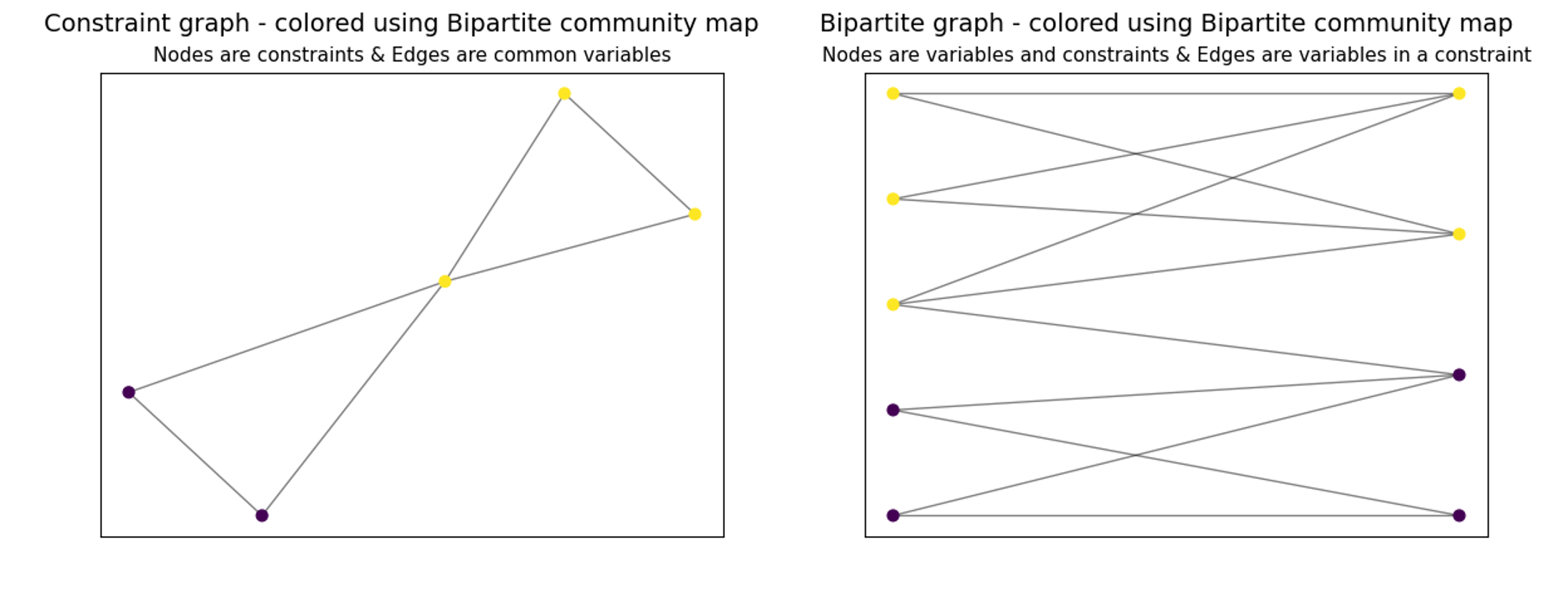
These graph drawings very clearly demonstrate the communities within this model. The constraint graph (which is colored using the bipartite community map) shows a very simple illustration - one node for each constraint, with only one edge connecting the two communities (which represents the variable m.x2 common to m.c2 and m.c3 in separate communities) The bipartite graph is slightly more complicated and we can see again how there is only one edge between the two communities and more edges within each community. This is an ideal situation for breaking a model into separate communities since there is little connectivity between the communities. Also, note that we can choose different graph types (such as a variable node graph, constraint node graph, or bipartite graph) for a given community map.

Let’s try a more complicated model (taken from Duran & Grossmann, 1986) - this example will demonstrate how the same graph can be illustrated using different community maps (in the previous example we illustrated different graphs with a single community map):

Define the model
>>> model = EightProcessFlowsheet()

Now, we follow steps similar to the example above (see above for explanations)
>>> community_map_object = cmo = detect_communities(model, type_of_community_map='constraint', random_seed=seed)
>>> left_fig, pos = cmo.visualize_model_graph(type_of_graph='variable')

As we did before, we will use the returned 'pos' to create a consistent graph layout
>>> community_map_object = cmo = detect_communities(model, type_of_community_map='bipartite')
>>> middle_fig, _ = cmo.visualize_model_graph(type_of_graph='variable', pos=pos)

>>> community_map_object = cmo = detect_communities(model, type_of_community_map='variable')
>>> right_fig, _ = cmo.visualize_model_graph(type_of_graph='variable', pos=pos)

We can see an example for the three separate graphs created by these three function calls below:

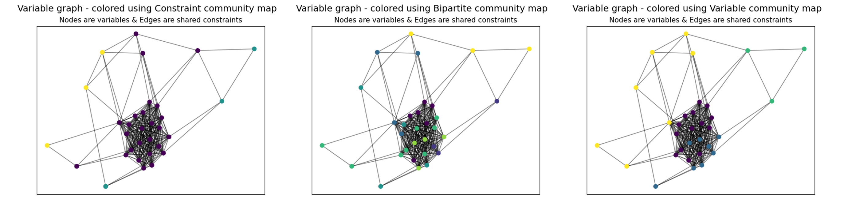
The three graphs above are all variable graphs - which means the nodes represent variables in the model, and the edges represent constraint equations. The coloring differs because the three graphs rely on community maps that were created based on a constraint node graph, a bipartite graph, and a variable node graph (from left to right). For example, the community map that was generated from a constraint node graph (type_of_community_map='constraint') resulted in three communities (as seen by the purple, yellow, and blue nodes).

generate_model_graph function

Now, we will take a look at generate_model_graph - this function can be used to create a NetworkX graph for a Pyomo model (and is used in detect_communities). Here, we will create a NetworkX graph from the model in our first example and then create the edge and adjacency list for the graph.

generate_model_graph returns three things:

• a NetworkX graph of the given model

• a dictionary that maps the numbers used to represent the model components to the actual components (because Pyomo components cannot be directly added to a NetworkX graph)

• a dictionary that maps constraints to the variables in them.

For this example, we will only need the NetworkX graph of the model and the number-to-component mapping.

Define the model
>>> model = decode_model_1()

See above for the description of the items returned by 'generate_model_graph'
>>> model_graph, number_component_map, constr_var_map = generate_model_graph(model, type_of_graph='constraint')

The next two lines create and implement a mapping to change the node values from numbers into
strings. The second line uses this mapping to create string_model_graph, which has
the relabeled nodes (strings instead of numbers).

>>> string_map = dict((number, str(comp)) for number, comp in number_component_map.items())
>>> string_model_graph = nx.relabel_nodes(model_graph, string_map)

Now, we print the edge list and the adjacency list:
Edge List:
>>> for line in nx.generate_edgelist(string_model_graph): print(line)  
c1 c2 {'weight': 2}
c1 c3 {'weight': 1}
c2 c3 {'weight': 1}
c3 c5 {'weight': 2}
c3 c4 {'weight': 2}
c4 c5 {'weight': 2}

Adjacency List:
>>> print(list(nx.generate_adjlist(string_model_graph)))  
['c1 c2 c3', 'c2 c3', 'c3 c5 c4', 'c4 c5', 'c5']

It’s worth mentioning that in the code above, we do not have to create string_map to create an edge list or adjacency list, but for the sake of having an easily understandable output, it is quite helpful. (Without relabeling the nodes, the output below would not have the strings of the components but instead would have integer values.) This code will hopefully make it easier for a user to do the same.

Functions in this Package

Main module for community detection integration with Pyomo models.

This module separates model components (variables, constraints, and objectives) into different communities distinguished by the degree of connectivity between community members.

Original implementation developed by Rahul Joglekar in the Grossmann research group.

class pyomo.contrib.community_detection.detection.CommunityMap(community_map, type_of_community_map, with_objective, weighted_graph, random_seed, use_only_active_components, model, graph, graph_node_mapping, constraint_variable_map, graph_partition)

This class is used to create CommunityMap objects which are returned by the detect_communities function. Instances of this class allow dict-like usage and store relevant information about the given community map, such as the model used to create them, their networkX representation, etc.

The CommunityMap object acts as a Python dictionary, mapping integer keys to tuples containing two lists (which contain the components in the given community) - a constraint list and variable list.

Methods: generate_structured_model visualize_model_graph

generate_structured_model()

Using the community map and the original model used to create this community map, we will create structured_model, which will be based on the original model but will place variables, constraints, and objectives into or outside of various blocks (communities) based on the community map.

Returns:

structured_model – a Pyomo model that reflects the nature of the community map

Return type:

Block

visualize_model_graph(type_of_graph='constraint', filename=None, pos=None)

This function draws a graph of the communities for a Pyomo model.

The type_of_graph parameter is used to create either a variable-node graph, constraint-node graph, or bipartite graph of the Pyomo model. Then, the nodes are colored based on the communities they are in - which is based on the community map (self.community_map). A filename can be provided to save the figure, otherwise the figure is illustrated with matplotlib.

Parameters:

• type_of_graph (str, optional) – a string that specifies the types of nodes drawn on the model graph, the default is ‘constraint’. ‘constraint’ draws a graph with constraint nodes, ‘variable’ draws a graph with variable nodes, ‘bipartite’ draws a bipartite graph (with both constraint and variable nodes)

• filename (str, optional) – a string that specifies a path for the model graph illustration to be saved

• pos (dict, optional) – a dictionary that maps node keys to their positions on the illustration

Returns:

• fig (matplotlib figure) – the figure for the model graph drawing

• pos (dict) – a dictionary that maps node keys to their positions on the illustration - can be used to create consistent layouts for graphs of a given model

pyomo.contrib.community_detection.detection.detect_communities(model, type_of_community_map='constraint', with_objective=True, weighted_graph=True, random_seed=None, use_only_active_components=True)

Detects communities in a Pyomo optimization model

This function takes in a Pyomo optimization model and organizes the variables and constraints into a graph of nodes and edges. Then, by using Louvain community detection on the graph, a dictionary (community_map) is created, which maps (arbitrary) community keys to the detected communities within the model.

Parameters:

• model (Block) – a Pyomo model or block to be used for community detection

• type_of_community_map (str, optional) – a string that specifies the type of community map to be returned, the default is ‘constraint’. ‘constraint’ returns a dictionary (community_map) with communities based on constraint nodes, ‘variable’ returns a dictionary (community_map) with communities based on variable nodes, ‘bipartite’ returns a dictionary (community_map) with communities based on a bipartite graph (both constraint and variable nodes)

• with_objective (bool, optional) – a Boolean argument that specifies whether or not the objective function is included in the model graph (and thus in ‘community_map’); the default is True

• weighted_graph (bool, optional) – a Boolean argument that specifies whether community_map is created based on a weighted model graph or an unweighted model graph; the default is True (type_of_community_map=’bipartite’ creates an unweighted model graph regardless of this parameter)

• random_seed (int, optional) – an integer that is used as the random seed for the (heuristic) Louvain community detection

• use_only_active_components (bool, optional) – a Boolean argument that specifies whether inactive constraints/objectives are included in the community map

Returns:

The CommunityMap object acts as a Python dictionary, mapping integer keys to tuples containing two lists (which contain the components in the given community) - a constraint list and variable list. Furthermore, the CommunityMap object stores relevant information about the given community map (dict), such as the model used to create it, its networkX representation, etc.

Return type:

CommunityMap object (dict-like object)

Model Graph Generator Code

pyomo.contrib.community_detection.community_graph.generate_model_graph(model, type_of_graph, with_objective=True, weighted_graph=True, use_only_active_components=True)

Creates a networkX graph of nodes and edges based on a Pyomo optimization model

This function takes in a Pyomo optimization model, then creates a graphical representation of the model with specific features of the graph determined by the user (see Parameters below).

(This function is designed to be called by detect_communities, but can be used solely for the purpose of creating model graphs as well.)

Parameters:

• model (Block) – a Pyomo model or block to be used for community detection

• type_of_graph (str) – a string that specifies the type of graph that is created from the model ‘constraint’ creates a graph based on constraint nodes, ‘variable’ creates a graph based on variable nodes, ‘bipartite’ creates a graph based on constraint and variable nodes (bipartite graph).

• with_objective (bool, optional) – a Boolean argument that specifies whether or not the objective function is included in the graph; the default is True

• weighted_graph (bool, optional) – a Boolean argument that specifies whether a weighted or unweighted graph is to be created from the Pyomo model; the default is True (type_of_graph=’bipartite’ creates an unweighted graph regardless of this parameter)

• use_only_active_components (bool, optional) – a Boolean argument that specifies whether inactive constraints/objectives are included in the networkX graph

Returns:

• bipartite_model_graph/projected_model_graph (nx.Graph) – a NetworkX graph with nodes and edges based on the given Pyomo optimization model

• number_component_map (dict) – a dictionary that (deterministically) maps a number to a component in the model

• constraint_variable_map (dict) – a dictionary that maps a numbered constraint to a list of (numbered) variables that appear in the constraint

Pyomo.DoE

Pyomo.DoE (Pyomo Design of Experiments) is a Python library for model-based design of experiments using science-based models.

Pyomo.DoE was developed by Jialu Wang and Alexander W. Dowling at the University of Notre Dame as part of the Carbon Capture Simulation for Industry Impact (CCSI2). project, funded through the U.S. Department Of Energy Office of Fossil Energy.

If you use Pyomo.DoE, please cite:

[Wang and Dowling, 2022] Wang, Jialu, and Alexander W. Dowling. “Pyomo.DOE: An open‐source package for model‐based design of experiments in Python.” AIChE Journal 68.12 (2022): e17813. https://doi.org/10.1002/aic.17813

Methodology Overview

Model-based Design of Experiments (MBDoE) is a technique to maximize the information gain of experiments by directly using science-based models with physically meaningful parameters. It is one key component in the model calibration and uncertainty quantification workflow shown below:

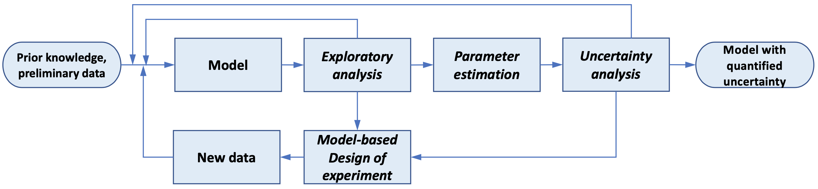
The exploratory analysis, parameter estimation, uncertainty analysis, and MBDoE are combined into an iterative framework to select, refine, and calibrate science-based mathematical models with quantified uncertainty. Currently, Pyomo.DoE focuses on increasing parameter precision.

Pyomo.DoE provides the exploratory analysis and MBDoE capabilities to the Pyomo ecosystem. The user provides one Pyomo model, a set of parameter nominal values, the allowable design spaces for design variables, and the assumed observation error model. During exploratory analysis, Pyomo.DoE checks if the model parameters can be inferred from the postulated measurements or preliminary data. MBDoE then recommends optimized experimental conditions for collecting more data. Parameter estimation packages such as Parmest can perform parameter estimation using the available data to infer values for parameters, and facilitate an uncertainty analysis to approximate the parameter covariance matrix. If the parameter uncertainties are sufficiently small, the workflow terminates and returns the final model with quantified parametric uncertainty. If not, MBDoE recommends optimized experimental conditions to generate new data.

Below is an overview of the type of optimization models Pyomo.DoE can accommodate:

• Pyomo.DoE is suitable for optimization models of continuous variables

• Pyomo.DoE can handle equality constraints defining state variables

• Pyomo.DoE supports (Partial) Differential-Algebraic Equations (PDAE) models via Pyomo.DAE

• Pyomo.DoE also supports models with only algebraic constraints

The general form of a DAE problem that can be passed into Pyomo.DoE is shown below:

\[\begin{split}\begin{align*} & \dot{\mathbf{x}}(t) = \mathbf{f}(\mathbf{x}(t), \mathbf{z}(t), \mathbf{y}(t), \mathbf{u}(t), \overline{\mathbf{w}}, \boldsymbol{\theta}) \\ & \mathbf{g}(\mathbf{x}(t), \mathbf{z}(t), \mathbf{y}(t), \mathbf{u}(t), \overline{\mathbf{w}},\boldsymbol{\theta})=\mathbf{0} \\ & \mathbf{y} =\mathbf{h}(\mathbf{x}(t), \mathbf{z}(t), \mathbf{u}(t), \overline{\mathbf{w}},\boldsymbol{\theta}) \\ & \mathbf{f}^{\mathbf{0}}\left(\dot{\mathbf{x}}\left(t_{0}\right), \mathbf{x}\left(t_{0}\right), \mathbf{z}(t_0), \mathbf{y}(t_0), \mathbf{u}\left(t_{0}\right), \overline{\mathbf{w}}, \boldsymbol{\theta})\right)=\mathbf{0} \\ & \mathbf{g}^{\mathbf{0}}\left( \mathbf{x}\left(t_{0}\right),\mathbf{z}(t_0), \mathbf{y}(t_0), \mathbf{u}\left(t_{0}\right), \overline{\mathbf{w}}, \boldsymbol{\theta}\right)=\mathbf{0}\\ &\mathbf{y}^{\mathbf{0}}\left(t_{0}\right)=\mathbf{h}\left(\mathbf{x}\left(t_{0}\right),\mathbf{z}(t_0), \mathbf{u}\left(t_{0}\right), \overline{\mathbf{w}}, \boldsymbol{\theta}\right) \end{align*}\end{split}\]

where:

• \(\boldsymbol{\theta} \in \mathbb{R}^{N_p}\) are unknown model parameters.

• \(\mathbf{x} \subseteq \mathcal{X}\) are dynamic state variables which characterize trajectory of the system, \(\mathcal{X} \in \mathbb{R}^{N_x \times N_t}\).

• \(\mathbf{z} \subseteq \mathcal{Z}\) are algebraic state variables, \(\mathcal{Z} \in \mathbb{R}^{N_z \times N_t}\).

• \(\mathbf{u} \subseteq \mathcal{U}\) are time-varying decision variables, \(\mathcal{U} \in \mathbb{R}^{N_u \times N_t}\).

• \(\overline{\mathbf{w}} \in \mathbb{R}^{N_w}\) are time-invariant decision variables.

• \(\mathbf{y} \subseteq \mathcal{Y}\) are measurement response variables, \(\mathcal{Y} \in \mathbb{R}^{N_r \times N_t}\).

• \(\mathbf{f}(\cdot)\) are differential equations.

• \(\mathbf{g}(\cdot)\) are algebraic equations.

• \(\mathbf{h}(\cdot)\) are measurement functions.

• \(\mathbf{t} \in \mathbb{R}^{N_t \times 1}\) is a union of all time sets.

Note

• Parameters and design variables should be defined as Pyomo Var components on the model to use direct_kaug mode, and can be defined as Pyomo Param object if not using direct_kaug.

Based on the above notation, the form of the MBDoE problem addressed in Pyomo.DoE is shown below:

\[\begin{split}\begin{equation} \begin{aligned} \underset{\boldsymbol{\varphi}}{\max} \quad & \Psi (\mathbf{M}(\mathbf{\hat{y}}, \boldsymbol{\varphi})) \\ \text{s.t.} \quad & \mathbf{M}(\boldsymbol{\hat{\theta}}, \boldsymbol{\varphi}) = \sum_r^{N_r} \sum_{r'}^{N_r} \tilde{\sigma}_{(r,r')}\mathbf{Q}_r^\mathbf{T} \mathbf{Q}_{r'} + \mathbf{V}^{-1}_{\boldsymbol{\theta}}(\boldsymbol{\hat{\theta}}) \\ & \dot{\mathbf{x}}(t) = \mathbf{f}(\mathbf{x}(t), \mathbf{z}(t), \mathbf{y}(t), \mathbf{u}(t), \overline{\mathbf{w}}, \boldsymbol{\theta}) \\ & \mathbf{g}(\mathbf{x}(t), \mathbf{z}(t), \mathbf{y}(t), \mathbf{u}(t), \overline{\mathbf{w}},\boldsymbol{\theta})=\mathbf{0} \\ & \mathbf{y} =\mathbf{h}(\mathbf{x}(t), \mathbf{z}(t), \mathbf{u}(t), \overline{\mathbf{w}},\boldsymbol{\theta}) \\ & \mathbf{f}^{\mathbf{0}}\left(\dot{\mathbf{x}}\left(t_{0}\right), \mathbf{x}\left(t_{0}\right), \mathbf{z}(t_0), \mathbf{y}(t_0), \mathbf{u}\left(t_{0}\right), \overline{\mathbf{w}}, \boldsymbol{\theta})\right)=\mathbf{0} \\ & \mathbf{g}^{\mathbf{0}}\left( \mathbf{x}\left(t_{0}\right),\mathbf{z}(t_0), \mathbf{y}(t_0), \mathbf{u}\left(t_{0}\right), \overline{\mathbf{w}}, \boldsymbol{\theta}\right)=\mathbf{0}\\ &\mathbf{y}^{\mathbf{0}}\left(t_{0}\right)=\mathbf{h}\left(\mathbf{x}\left(t_{0}\right),\mathbf{z}(t_0), \mathbf{u}\left(t_{0}\right), \overline{\mathbf{w}}, \boldsymbol{\theta}\right) \end{aligned} \end{equation}\end{split}\]

where:

• \(\boldsymbol{\varphi}\) are design variables, which are manipulated to maximize the information content of experiments. It should consist of one or more of \(\mathbf{u}(t), \mathbf{y}^{\mathbf{0}}({t_0}),\overline{\mathbf{w}}\). With a proper model formulation, the timepoints for control or measurements \(\mathbf{t}\) can also be degrees of freedom.

• \(\mathbf{M}\) is the Fisher information matrix (FIM), estimated as the inverse of the covariance matrix of parameter estimates \(\boldsymbol{\hat{\theta}}\). A large FIM indicates more information contained in the experiment for parameter estimation.

• \(\mathbf{Q}\) is the dynamic sensitivity matrix, containing the partial derivatives of \(\mathbf{y}\) with respect to \(\boldsymbol{\theta}\).

• \(\Psi\) is the design criteria to measure FIM.

• \(\mathbf{V}_{\boldsymbol{\theta}}(\boldsymbol{\hat{\theta}})^{-1}\) is the FIM of previous experiments.

Pyomo.DoE provides four design criteria \(\Psi\) to measure the size of FIM:

Pyomo.DoE design criteria

Design criterion	Computation	Geometrical meaning
A-optimality	\(\text{trace}({\mathbf{M}})\)	Dimensions of the enclosing box of the confidence ellipse
D-optimality	\(\text{det}({\mathbf{M}})\)	Volume of the confidence ellipse
E-optimality	\(\text{min eig}({\mathbf{M}})\)	Size of the longest axis of the confidence ellipse
Modified E-optimality	\(\text{cond}({\mathbf{M}})\)	Ratio of the longest axis to the shortest axis of the confidence ellipse

In order to solve problems of the above, Pyomo.DoE implements the 2-stage stochastic program. Please see Wang and Dowling (2022) for details.

Pyomo.DoE Required Inputs

The required input to the Pyomo.DoE solver is an Experiment object. The experiment object must have a get_labeled_model function which returns a Pyomo model with four Suffix components identifying the parts of the model used in MBDoE analysis. This is in line with the convention used in the parameter estimation tool, Parmest. The four Suffix components are:

• experiment_inputs - The experimental design decisions

• experiment_outputs - The values measured during the experiment

• measurement_error - The error associated with individual values measured during the experiment

• unknown_parameters - Those parameters in the model that are estimated using the measured values during the experiment

An example Experiment object that builds and labels the model is shown in the next few sections.

Pyomo.DoE Usage Example

We illustrate the use of Pyomo.DoE using a reaction kinetics example (Wang and Dowling, 2022). The Arrhenius equations model the temperature dependence of the reaction rate coefficient \(k_1, k_2\). Assuming a first-order reaction mechanism gives the reaction rate model. Further, we assume only species A is fed to the reactor.

\[\begin{split}\begin{equation} \begin{aligned} k_1 & = A_1 e^{-\frac{E_1}{RT}} \\ k_2 & = A_2 e^{-\frac{E_2}{RT}} \\ \frac{d{C_A}}{dt} & = -k_1{C_A} \\ \frac{d{C_B}}{dt} & = k_1{C_A} - k_2{C_B} \\ C_{A0}& = C_A + C_B + C_C \\ C_B(t_0) & = 0 \\ C_C(t_0) & = 0 \\ \end{aligned} \end{equation}\end{split}\]

\(C_A(t), C_B(t), C_C(t)\) are the time-varying concentrations of the species A, B, C, respectively. \(k_1, k_2\) are the rates for the two chemical reactions using an Arrhenius equation with activation energies \(E_1, E_2\) and pre-exponential factors \(A_1, A_2\). The goal of MBDoE is to optimize the experiment design variables \(\boldsymbol{\varphi} = (C_{A0}, T(t))\), where \(C_{A0},T(t)\) are the initial concentration of species A and the time-varying reactor temperature, to maximize the precision of unknown model parameters \(\boldsymbol{\theta} = (A_1, E_1, A_2, E_2)\) by measuring \(\mathbf{y}(t)=(C_A(t), C_B(t), C_C(t))\). The observation errors are assumed to be independent both in time and across measurements with a constant standard deviation of 1 M for each species.

Step 0: Import Pyomo and the Pyomo.DoE module and create an Experiment class

>>> # === Required import ===
>>> import pyomo.environ as pyo
>>> from pyomo.contrib.doe import DesignOfExperiments
>>> import numpy as np

class ReactorExperiment(Experiment):
    def __init__(self, data, nfe, ncp):
        """
        Arguments
        ---------
        data: object containing vital experimental information
        nfe: number of finite elements
        ncp: number of collocation points for the finite elements
        """
        self.data = data
        self.nfe = nfe
        self.ncp = ncp
        self.model = None

        #############################

Step 1: Define the Pyomo process model

The process model for the reaction kinetics problem is shown below. We build the model without any data or discretization.

    def create_model(self):
        """
        This is an example user model provided to DoE library.
        It is a dynamic problem solved by Pyomo.DAE.

        Return
        ------
        m: a Pyomo.DAE model
        """

        m = self.model = pyo.ConcreteModel()

        # Model parameters
        m.R = pyo.Param(mutable=False, initialize=8.314)

        # Define model variables
        ########################
        # time
        m.t = ContinuousSet(bounds=[0, 1])

        # Concentrations
        m.CA = pyo.Var(m.t, within=pyo.NonNegativeReals)
        m.CB = pyo.Var(m.t, within=pyo.NonNegativeReals)
        m.CC = pyo.Var(m.t, within=pyo.NonNegativeReals)

        # Temperature
        m.T = pyo.Var(m.t, within=pyo.NonNegativeReals)

        # Arrhenius rate law equations
        m.A1 = pyo.Var(within=pyo.NonNegativeReals)
        m.E1 = pyo.Var(within=pyo.NonNegativeReals)
        m.A2 = pyo.Var(within=pyo.NonNegativeReals)
        m.E2 = pyo.Var(within=pyo.NonNegativeReals)

        # Differential variables (Conc.)
        m.dCAdt = DerivativeVar(m.CA, wrt=m.t)
        m.dCBdt = DerivativeVar(m.CB, wrt=m.t)

        ########################
        # End variable def.

        # Equation definition
        ########################

        # Expression for rate constants
        @m.Expression(m.t)
        def k1(m, t):
            return m.A1 * pyo.exp(-m.E1 * 1000 / (m.R * m.T[t]))

        @m.Expression(m.t)
        def k2(m, t):
            return m.A2 * pyo.exp(-m.E2 * 1000 / (m.R * m.T[t]))

        # Concentration odes
        @m.Constraint(m.t)
        def CA_rxn_ode(m, t):
            return m.dCAdt[t] == -m.k1[t] * m.CA[t]

        @m.Constraint(m.t)
        def CB_rxn_ode(m, t):
            return m.dCBdt[t] == m.k1[t] * m.CA[t] - m.k2[t] * m.CB[t]

        # algebraic balance for concentration of C
        # Valid because the reaction system (A --> B --> C) is equimolar
        @m.Constraint(m.t)
        def CC_balance(m, t):
            return m.CA[0] == m.CA[t] + m.CB[t] + m.CC[t]

        ########################

Step 2: Finalize the Pyomo process model

Here we add data to the model and finalize the discretization. This step is required before the model can be labeled.

    def finalize_model(self):
        """
        Example finalize model function. There are two main tasks
        here:
            1. Extracting useful information for the model to align
               with the experiment. (Here: CA0, t_final, t_control)
            2. Discretizing the model subject to this information.
        """
        m = self.model

        # Unpacking data before simulation
        control_points = self.data["control_points"]

        # Set initial concentration values for the experiment
        m.CA[0].value = self.data["CA0"]
        m.CB[0].fix(self.data["CB0"])

        # Update model time `t` with time range and control time points
        m.t.update(self.data["t_range"])
        m.t.update(control_points)

        # Fix the unknown parameter values
        m.A1.fix(self.data["A1"])
        m.A2.fix(self.data["A2"])
        m.E1.fix(self.data["E1"])
        m.E2.fix(self.data["E2"])

        # Add upper and lower bounds to the design variable, CA[0]
        m.CA[0].setlb(self.data["CA_bounds"][0])
        m.CA[0].setub(self.data["CA_bounds"][1])

        m.t_control = control_points

        # Discretizing the model
        discr = pyo.TransformationFactory("dae.collocation")
        discr.apply_to(m, nfe=self.nfe, ncp=self.ncp, wrt=m.t)

        # Initializing Temperature in the model
        cv = None
        for t in m.t:
            if t in control_points:
                cv = control_points[t]
            m.T[t].setlb(self.data["T_bounds"][0])
            m.T[t].setub(self.data["T_bounds"][1])
            m.T[t] = cv

        # Make a constraint that holds temperature constant between control time points
        @m.Constraint(m.t - control_points)
        def T_control(m, t):
            """
            Piecewise constant temperature between control points
            """
            neighbour_t = max(tc for tc in control_points if tc < t)
            return m.T[t] == m.T[neighbour_t]

        #########################

Step 3: Label the information needed for DoE analysis

We label the four important groups as defined before.

    def label_experiment(self):
        """
        Example for annotating (labeling) the model with a
        full experiment.
        """
        m = self.model

        # Set measurement labels
        m.experiment_outputs = pyo.Suffix(direction=pyo.Suffix.LOCAL)
        # Add CA to experiment outputs
        m.experiment_outputs.update((m.CA[t], None) for t in m.t_control)
        # Add CB to experiment outputs
        m.experiment_outputs.update((m.CB[t], None) for t in m.t_control)
        # Add CC to experiment outputs
        m.experiment_outputs.update((m.CC[t], None) for t in m.t_control)

        # Adding error for measurement values (assuming no covariance and constant error for all measurements)
        m.measurement_error = pyo.Suffix(direction=pyo.Suffix.LOCAL)
        concentration_error = 1e-2  # Error in concentration measurement
        # Add measurement error for CA
        m.measurement_error.update((m.CA[t], concentration_error) for t in m.t_control)
        # Add measurement error for CB
        m.measurement_error.update((m.CB[t], concentration_error) for t in m.t_control)
        # Add measurement error for CC
        m.measurement_error.update((m.CC[t], concentration_error) for t in m.t_control)

        # Identify design variables (experiment inputs) for the model
        m.experiment_inputs = pyo.Suffix(direction=pyo.Suffix.LOCAL)
        # Add experimental input label for initial concentration
        m.experiment_inputs[m.CA[m.t.first()]] = None
        # Add experimental input label for Temperature
        m.experiment_inputs.update((m.T[t], None) for t in m.t_control)

        # Add unknown parameter labels
        m.unknown_parameters = pyo.Suffix(direction=pyo.Suffix.LOCAL)
        # Add labels to all unknown parameters with nominal value as the value
        m.unknown_parameters.update((k, pyo.value(k)) for k in [m.A1, m.A2, m.E1, m.E2])

        #########################

Step 4: Implement the get_labeled_model method

This method utilizes the previous 3 steps and is used by Pyomo.DoE to build the model to perform optimal experimental design.

    def get_labeled_model(self):
        if self.model is None:
            self.create_model()
            self.finalize_model()
            self.label_experiment()
        return self.model

Step 5: Exploratory analysis (Enumeration)

Exploratory analysis is suggested to enumerate the design space to check if the problem is identifiable, i.e., ensure that D-, E-optimality metrics are not small numbers near zero, and Modified E-optimality is not a big number.

Pyomo.DoE can perform exploratory sensitivity analysis with the compute_FIM_full_factorial function. The compute_FIM_full_factorial function generates a grid over the design space as specified by the user. Each grid point represents an MBDoE problem solved using compute_FIM method. In this way, sensitivity of the FIM over the design space can be evaluated.

The following code executes the above problem description:

    DATA_DIR = Path(__file__).parent
    file_path = DATA_DIR / "result.json"

    with open(file_path) as f:
        data_ex = json.load(f)

    # Put temperature control time points into correct format for reactor experiment
    data_ex["control_points"] = {
        float(k): v for k, v in data_ex["control_points"].items()
    }

    # Create a ReactorExperiment object; data and discretization information are part
    # of the constructor of this object
    experiment = ReactorExperiment(data=data_ex, nfe=10, ncp=3)

    # Use a central difference, with step size 1e-3
    fd_formula = "central"
    step_size = 1e-3

    # Use the determinant objective with scaled sensitivity matrix
    objective_option = "determinant"
    scale_nominal_param_value = True

    # Create the DesignOfExperiments object
    # We will not be passing any prior information in this example
    # and allow the experiment object and the DesignOfExperiments
    # call of ``run_doe`` perform model initialization.
    doe_obj = DesignOfExperiments(
        experiment,
        fd_formula=fd_formula,
        step=step_size,
        objective_option=objective_option,
        scale_constant_value=1,
        scale_nominal_param_value=scale_nominal_param_value,
        prior_FIM=None,
        jac_initial=None,
        fim_initial=None,
        L_diagonal_lower_bound=1e-7,
        solver=None,
        tee=False,
        get_labeled_model_args=None,
        _Cholesky_option=True,
        _only_compute_fim_lower=True,
    )

    # Make design ranges to compute the full factorial design
    design_ranges = {"CA[0]": [1, 5, 9], "T[0]": [300, 700, 9]}

    # Compute the full factorial design with the sequential FIM calculation
    doe_obj.compute_FIM_full_factorial(design_ranges=design_ranges, method="sequential")

    # Plot the results
    doe_obj.draw_factorial_figure(
        sensitivity_design_variables=["CA[0]", "T[0]"],
        fixed_design_variables={
            "T[0.125]": 300,
            "T[0.25]": 300,
            "T[0.375]": 300,
            "T[0.5]": 300,
            "T[0.625]": 300,
            "T[0.75]": 300,
            "T[0.875]": 300,
            "T[1]": 300,
        },
        title_text="Reactor Example",
        xlabel_text="Concentration of A (M)",
        ylabel_text="Initial Temperature (K)",
        figure_file_name="example_reactor_compute_FIM",
        log_scale=False,
    )

    ###########################

An example output of the code above, a design exploration for the initial concentration and temperature as experimental design variables with 9 values, produces the four figures summarized below:

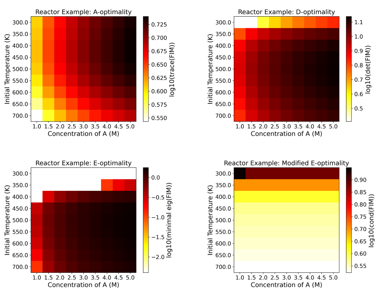
A heatmap shows the change of the objective function, a.k.a. the experimental information content, in the design space. Horizontal and vertical axes are the two experimental design variables, while the color of each grid shows the experimental information content. For A optimality (top left subfigure), the figure shows that the most informative region is around \(C_{A0}=5.0\) M, \(T=300.0\) K, while the least informative region is around \(C_{A0}=1.0\) M, \(T=700.0\) K.

Step 6: Performing an optimal experimental design

In step 5, the DoE object was constructed to perform an exploratory sensitivity analysis. The same object can be used to design an optimal experiment with a single line of code.

    ####################
    doe_obj.run_doe()

When run, the optimal design is an initial concentration of 5.0 mol/L and an initial temperature of 494 K with all other temperatures being 300 K. The corresponding log-10 determinant of the FIM is 13.75

GDPopt logic-based solver

The GDPopt solver in Pyomo allows users to solve nonlinear Generalized Disjunctive Programming (GDP) models using logic-based decomposition approaches, as opposed to the conventional approach via reformulation to a Mixed Integer Nonlinear Programming (MINLP) model.

The main advantage of these techniques is their ability to solve subproblems in a reduced space, including nonlinear constraints only for True logical blocks. As a result, GDPopt is most effective for nonlinear GDP models.

Three algorithms are available in GDPopt:

1. Logic-based outer approximation (LOA) [Turkay & Grossmann, 1996]

2. Global logic-based outer approximation (GLOA) [Lee & Grossmann, 2001]

3. Logic-based branch-and-bound (LBB) [Lee & Grossmann, 2001]

Usage and implementation details for GDPopt can be found in the PSE 2018 paper (Chen et al., 2018), or via its preprint.

Credit for prototyping and development can be found in the GDPopt class documentation, below.

GDPopt can be used to solve a Pyomo.GDP concrete model in two ways. The simplest is to instantiate the generic GDPopt solver and specify the desired algorithm as an argument to the solve method:

>>> SolverFactory('gdpopt').solve(model, algorithm='LOA')

The alternative is to instantiate an algorithm-specific GDPopt solver:

>>> SolverFactory('gdpopt.loa').solve(model)

In the above examples, GDPopt uses the GDPopt-LOA algorithm. Other algorithms may be used by specifying them in the algorithm argument when using the generic solver or by instantiating the algorithm-specific GDPopt solvers. All GDPopt options are listed below.

Note

The generic GDPopt solver allows minimal configuration outside of the arguments to the solve method. To avoid repeatedly specifying the same configuration options to the solve method, use the algorithm-specific solvers.

Logic-based Outer Approximation (LOA)

Chen et al., 2018 contains the following flowchart, taken from the preprint version:

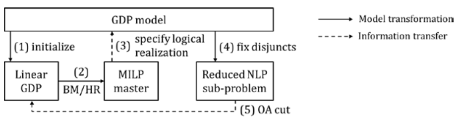
An example that includes the modeling approach may be found below.

Required imports
>>> from pyomo.environ import *
>>> from pyomo.gdp import *

Create a simple model
>>> model = ConcreteModel(name='LOA example')

>>> model.x = Var(bounds=(-1.2, 2))
>>> model.y = Var(bounds=(-10,10))
>>> model.c = Constraint(expr= model.x + model.y == 1)

>>> model.fix_x = Disjunct()
>>> model.fix_x.c = Constraint(expr=model.x == 0)

>>> model.fix_y = Disjunct()
>>> model.fix_y.c = Constraint(expr=model.y == 0)

>>> model.d = Disjunction(expr=[model.fix_x, model.fix_y])
>>> model.objective = Objective(expr=model.x + 0.1*model.y, sense=minimize)

Solve the model using GDPopt
>>> results = SolverFactory('gdpopt.loa').solve(
...     model, mip_solver='glpk') 

Display the final solution
>>> model.display()
Model LOA example

  Variables:
    x : Size=1, Index=None
        Key  : Lower : Value : Upper : Fixed : Stale : Domain
        None :  -1.2 :     0 :     2 : False : False :  Reals
    y : Size=1, Index=None
        Key  : Lower : Value : Upper : Fixed : Stale : Domain
        None :   -10 :     1 :    10 : False : False :  Reals

  Objectives:
    objective : Size=1, Index=None, Active=True
        Key  : Active : Value
        None :   True :   0.1

  Constraints:
    c : Size=1
        Key  : Lower : Body : Upper
        None :   1.0 :    1 :   1.0

Note

When troubleshooting, it can often be helpful to turn on verbose output using the tee flag.

>>> SolverFactory('gdpopt.loa').solve(model, tee=True)

Global Logic-based Outer Approximation (GLOA)

The same algorithm can be used to solve GDPs involving nonconvex nonlinear constraints by solving the subproblems globally:

>>> SolverFactory('gdpopt.gloa').solve(model)

Warning

The nlp_solver option must be set to a global solver for the solution returned by GDPopt to also be globally optimal.

Relaxation with Integer Cuts (RIC)

Instead of outer approximation, GDPs can be solved using the same MILP relaxation as in the previous two algorithms, but instead of using the subproblems to generate outer-approximation cuts, the algorithm adds only no-good cuts for every discrete solution encountered:

>>> SolverFactory('gdpopt.ric').solve(model)

Again, this is a global algorithm if the subproblems are solved globally, and is not otherwise.

Note

The RIC algorithm will not necessarily enumerate all discrete solutions as it is possible for the bounds to converge first. However, full enumeration is not uncommon.

Logic-based Branch-and-Bound (LBB)

The GDPopt-LBB solver branches through relaxed subproblems with inactive disjunctions. It explores the possibilities based on best lower bound, eventually activating all disjunctions and presenting the globally optimal solution.

To use the GDPopt-LBB solver, define your Pyomo GDP model as usual:

Required imports
>>> from pyomo.environ import *
>>> from pyomo.gdp import Disjunct, Disjunction

Create a simple model
>>> m = ConcreteModel()
>>> m.x1 = Var(bounds = (0,8))
>>> m.x2 = Var(bounds = (0,8))
>>> m.obj = Objective(expr=m.x1 + m.x2, sense=minimize)
>>> m.y1 = Disjunct()
>>> m.y2 = Disjunct()
>>> m.y1.c1 = Constraint(expr=m.x1 >= 2)
>>> m.y1.c2 = Constraint(expr=m.x2 >= 2)
>>> m.y2.c1 = Constraint(expr=m.x1 >= 3)
>>> m.y2.c2 = Constraint(expr=m.x2 >= 3)
>>> m.djn = Disjunction(expr=[m.y1, m.y2])

Invoke the GDPopt-LBB solver

>>> results = SolverFactory('gdpopt.lbb').solve(m)
WARNING: 09/06/22: The GDPopt LBB algorithm currently has known issues. Please
    use the results with caution and report any bugs!

>>> print(results)  
>>> print(results.solver.status)
ok
>>> print(results.solver.termination_condition)
optimal

>>> print([value(m.y1.indicator_var), value(m.y2.indicator_var)])
[True, False]

GDPopt implementation and optional arguments

Warning

GDPopt optional arguments should be considered beta code and are subject to change.

class pyomo.contrib.gdpopt.GDPopt.GDPoptSolver

Decomposition solver for Generalized Disjunctive Programming (GDP) problems.

The GDPopt (Generalized Disjunctive Programming optimizer) solver applies a variety of decomposition-based approaches to solve Generalized Disjunctive Programming (GDP) problems. GDP models can include nonlinear, continuous variables and constraints, as well as logical conditions.

These approaches include:

• Logic-based outer approximation (LOA)

• Logic-based branch-and-bound (LBB)

• Partial surrogate cuts [pending]

• Generalized Bender decomposition [pending]

This solver implementation was developed by Carnegie Mellon University in the research group of Ignacio Grossmann.

For nonconvex problems, LOA may not report rigorous lower/upper bounds.

Questions: Please make a post at StackOverflow and/or contact Qi Chen <https://github.com/qtothec> or David Bernal <https://github.com/bernalde>.

Several key GDPopt components were prototyped by BS and MS students:

• Logic-based branch and bound: Sunjeev Kale

• MC++ interface: Johnny Bates

• LOA set-covering initialization: Eloy Fernandez

• Logic-to-linear transformation: Romeo Valentin

available(exception_flag=True)

Solver is always available. Though subsolvers may not be, they will raise an error when the time comes.

solve(model, **kwds)

Solve the model.

Parameters:

model (Block) – a Pyomo model or block to be solved

Keyword Arguments:

• iterlim (NonNegativeInt, optional) – Iteration limit.

• time_limit (PositiveInt, optional) – Seconds allowed until terminated. Note that the time limit can currently only be enforced between subsolver invocations. You may need to set subsolver time limits as well.

• tee (bool, default=False) – Stream output to terminal.

• logger (a_logger, default='pyomo.contrib.gdpopt') – The logger object or name to use for reporting.

version()

Return a 3-tuple describing the solver version.

class pyomo.contrib.gdpopt.loa.GDP_LOA_Solver(**kwds)

The GDPopt (Generalized Disjunctive Programming optimizer) logic-based outer approximation (LOA) solver.

Accepts models that can include nonlinear, continuous variables and constraints, as well as logical conditions. For nonconvex problems, LOA may not report rigorous dual bounds.

solve(model, **kwds)

Solve the model.

Parameters:

model (Block) – the Pyomo model or block to be solved

Keyword Arguments:

• iterlim (NonNegativeInt, optional) – Iteration limit.

• time_limit (PositiveInt, optional) – Seconds allowed until terminated. Note that the time limit can currently only be enforced between subsolver invocations. You may need to set subsolver time limits as well.

• tee (bool, default=False) – Stream output to terminal.

• logger (a_logger, default=<Logger pyomo.contrib.gdpopt (WARNING)>) – The logger object or name to use for reporting.

• integer_tolerance (default=1e-05) – Tolerance on integral values.

• constraint_tolerance (default=1e-06) –

  Tolerance on constraint satisfaction.

  Increasing this tolerance corresponds to being more conservative in declaring the model or an NLP subproblem to be infeasible.

• variable_tolerance (default=1e-08) – Tolerance on variable bounds.

• subproblem_initialization_method (default=<function restore_vars_to_original_values at 0x7f2a23c70f70>) –

  Callback to specify custom routines for initializing the (MI)NLP subproblems. This method is called after the discrete problem solution is fixed in the subproblem and before the subproblem is solved (or pre-solved).

  For algorithms with a discrete problem relaxation: This method accepts three arguments: the solver object, the subproblem GDPopt utility block and the discrete problem GDPopt utility block. The discrete problem contains the most recent discrete problem solution.

  For algorithms without a discrete problem relaxation: This method accepts four arguments: the list of Disjuncts that are currently fixed as being active, a list of values for the non-indicator BooleanVars (empty if force_nlp_subproblem=False), and a list of values for the integer vars (also empty if force_nlp_subproblem=False), and last the subproblem GDPopt utility block.

  The return of this method will be unused: The method should directly set the value of the variables on the subproblem

• call_before_subproblem_solve (default=<class 'pyomo.contrib.gdpopt.util._DoNothing'>) –

  Callback called right before the (MI)NLP subproblem is solved. Takes three arguments: The solver object, the subproblem and the GDPopt utility block on the subproblem.

  Note that unless you are very confident in what you are doing, the subproblem should not be modified in this callback: it should be used to interrogate the problem only.

  To initialize the problem before it is solved, please specify a method in the ‘subproblem_initialization_method’ argument.

• call_after_subproblem_solve (default=<class 'pyomo.contrib.gdpopt.util._DoNothing'>) –

  Callback called right after the (MI)NLP subproblem is solved. Takes three arguments: The solver object, the subproblem, and the GDPopt utility block on the subproblem.

  Note that unless you are very confident in what you are doing, the subproblem should not be modified in this callback: it should be used to interrogate the problem only.

• call_after_subproblem_feasible (default=<class 'pyomo.contrib.gdpopt.util._DoNothing'>) –

  Callback called right after the (MI)NLP subproblem is solved, if it was feasible. Takes three arguments: The solver object, the subproblem and the GDPopt utility block on the subproblem.

  Note that unless you are very confident in what you are doing, the subproblem should not be modified in this callback: it should be used to interrogate the problem only.

• force_subproblem_nlp (default=False) – Force subproblems to be NLP, even if discrete variables exist.

• subproblem_presolve (bool, default=True) – Flag to enable or disable subproblem presolve. Default=True.

• tighten_nlp_var_bounds (bool, default=False) – Whether or not to do feasibility-based bounds tightening on the variables in the NLP subproblem before solving it.

• round_discrete_vars (default=True) – Flag to round subproblem discrete variable values to the nearest integer. Rounding is done before fixing disjuncts.

• max_fbbt_iterations (PositiveInt, default=3) – Maximum number of feasibility-based bounds tightening iterations to do during NLP subproblem preprocessing.

• init_strategy (_init_strategy_deprecation, optional) – DEPRECATED: Please use ‘init_algorithm’ instead.

• init_algorithm (In{'no_init': <class 'pyomo.contrib.gdpopt.util._DoNothing'>, 'set_covering': <function init_set_covering at 0x7f2a23c70dc0>, 'max_binary': <function init_max_binaries at 0x7f2a23c70b80>, 'fix_disjuncts': <function init_fixed_disjuncts at 0x7f2a23c709d0>, 'custom_disjuncts': <function init_custom_disjuncts at 0x7f2a23c70940>}, default='set_covering') – Selects the initialization algorithm to use when generating the initial cuts to construct the discrete problem.

• custom_init_disjuncts (optional) – List of disjunct sets to use for initialization.

• max_slack (NonNegativeFloat, default=1000) – Upper bound on slack variables for OA

• OA_penalty_factor (NonNegativeFloat, default=1000) – Penalty multiplication term for slack variables on the objective value.

• set_cover_iterlim (NonNegativeInt, default=8) – Limit on the number of set covering iterations.

• discrete_problem_transformation (default='gdp.bigm') – Name of the transformation to use to transform the discrete problem from a GDP to an algebraic model.

• call_before_discrete_problem_solve (default=<class 'pyomo.contrib.gdpopt.util._DoNothing'>) –

  Callback called right before the MILP discrete problem is solved. Takes three arguments: The solver object, the discrete problem, and the GDPopt utility block on the discrete problem.

  Note that unless you are very confident in what you are doing, the problem should not be modified in this callback: it should be used to interrogate the problem only.

• call_after_discrete_problem_solve (default=<class 'pyomo.contrib.gdpopt.util._DoNothing'>) –

  Callback called right after the MILP discrete problem is solved. Takes three arguments: The solver object, the discrete problem, and the GDPopt utility block on the discrete problem.

  Note that unless you are very confident in what you are doing, the problem should not be modified in this callback: it should be used to interrogate the problem only.

• call_before_master_solve (default=<class 'pyomo.contrib.gdpopt.util._DoNothing'>) – DEPRECATED: Please use ‘call_before_discrete_problem_solve’

• call_after_master_solve (default=<class 'pyomo.contrib.gdpopt.util._DoNothing'>) – DEPRECATED: Please use ‘call_after_discrete_problem_solve’

• mip_presolve (bool, default=True) – Flag to enable or disable GDPopt MIP presolve. Default=True.

• calc_disjunctive_bounds (bool, default=False) – Calculate special disjunctive variable bounds for GLOA. False by default.

• obbt_disjunctive_bounds (bool, default=False) – Use optimality-based bounds tightening rather than feasibility-based bounds tightening to compute disjunctive variable bounds. False by default.

• mip_solver (default='gurobi') – Mixed-integer linear solver to use. Note that no persisent solvers other than the auto-persistent solvers in the APPSI package are supported.

• mip_solver_args (dict, optional) – Keyword arguments to send to the MILP subsolver solve() invocation

• nlp_solver (default='ipopt') – Nonlinear solver to use. Note that no persisent solvers other than the auto-persistent solvers in the APPSI package are supported.

• nlp_solver_args (dict, optional) – Keyword arguments to send to the NLP subsolver solve() invocation

• minlp_solver (default='baron') – Mixed-integer nonlinear solver to use. Note that no persisent solvers other than the auto-persistent solvers in the APPSI package are supported.

• minlp_solver_args (dict, optional) – Keyword arguments to send to the MINLP subsolver solve() invocation

• local_minlp_solver (default='bonmin') – Mixed-integer nonlinear solver to use. Note that no persisent solvers other than the auto-persistent solvers in the APPSI package are supported.

• local_minlp_solver_args (dict, optional) – Keyword arguments to send to the local MINLP subsolver solve() invocation

• small_dual_tolerance (default=1e-08) – When generating cuts, small duals multiplied by expressions can cause problems. Exclude all duals smaller in absolute value than the following.

• bound_tolerance (NonNegativeFloat, default=1e-06) – Tolerance for bound convergence.

class pyomo.contrib.gdpopt.gloa.GDP_GLOA_Solver(**kwds)

The GDPopt (Generalized Disjunctive Programming optimizer) global logic-based outer approximation (GLOA) solver.

Accepts models that can include nonlinear, continuous variables and constraints, as well as logical conditions.

solve(model, **kwds)

Solve the model.

Parameters:

model (Block) – the Pyomo model or block to be solved

Keyword Arguments:

• iterlim (NonNegativeInt, optional) – Iteration limit.

• time_limit (PositiveInt, optional) – Seconds allowed until terminated. Note that the time limit can currently only be enforced between subsolver invocations. You may need to set subsolver time limits as well.

• tee (bool, default=False) – Stream output to terminal.

• logger (a_logger, default=<Logger pyomo.contrib.gdpopt (WARNING)>) – The logger object or name to use for reporting.

• integer_tolerance (default=1e-05) – Tolerance on integral values.

• constraint_tolerance (default=1e-06) –

  Tolerance on constraint satisfaction.

  Increasing this tolerance corresponds to being more conservative in declaring the model or an NLP subproblem to be infeasible.

• variable_tolerance (default=1e-08) – Tolerance on variable bounds.

• subproblem_initialization_method (default=<function restore_vars_to_original_values at 0x7f2a23c70f70>) –

  Callback to specify custom routines for initializing the (MI)NLP subproblems. This method is called after the discrete problem solution is fixed in the subproblem and before the subproblem is solved (or pre-solved).

  For algorithms with a discrete problem relaxation: This method accepts three arguments: the solver object, the subproblem GDPopt utility block and the discrete problem GDPopt utility block. The discrete problem contains the most recent discrete problem solution.

  For algorithms without a discrete problem relaxation: This method accepts four arguments: the list of Disjuncts that are currently fixed as being active, a list of values for the non-indicator BooleanVars (empty if force_nlp_subproblem=False), and a list of values for the integer vars (also empty if force_nlp_subproblem=False), and last the subproblem GDPopt utility block.

  The return of this method will be unused: The method should directly set the value of the variables on the subproblem

• call_before_subproblem_solve (default=<class 'pyomo.contrib.gdpopt.util._DoNothing'>) –

  Callback called right before the (MI)NLP subproblem is solved. Takes three arguments: The solver object, the subproblem and the GDPopt utility block on the subproblem.

  Note that unless you are very confident in what you are doing, the subproblem should not be modified in this callback: it should be used to interrogate the problem only.

  To initialize the problem before it is solved, please specify a method in the ‘subproblem_initialization_method’ argument.

• call_after_subproblem_solve (default=<class 'pyomo.contrib.gdpopt.util._DoNothing'>) –

  Callback called right after the (MI)NLP subproblem is solved. Takes three arguments: The solver object, the subproblem, and the GDPopt utility block on the subproblem.

  Note that unless you are very confident in what you are doing, the subproblem should not be modified in this callback: it should be used to interrogate the problem only.

• call_after_subproblem_feasible (default=<class 'pyomo.contrib.gdpopt.util._DoNothing'>) –

  Callback called right after the (MI)NLP subproblem is solved, if it was feasible. Takes three arguments: The solver object, the subproblem and the GDPopt utility block on the subproblem.

  Note that unless you are very confident in what you are doing, the subproblem should not be modified in this callback: it should be used to interrogate the problem only.

• force_subproblem_nlp (default=False) – Force subproblems to be NLP, even if discrete variables exist.

• subproblem_presolve (bool, default=True) – Flag to enable or disable subproblem presolve. Default=True.

• tighten_nlp_var_bounds (bool, default=False) – Whether or not to do feasibility-based bounds tightening on the variables in the NLP subproblem before solving it.

• round_discrete_vars (default=True) – Flag to round subproblem discrete variable values to the nearest integer. Rounding is done before fixing disjuncts.

• max_fbbt_iterations (PositiveInt, default=3) – Maximum number of feasibility-based bounds tightening iterations to do during NLP subproblem preprocessing.

• init_strategy (_init_strategy_deprecation, optional) – DEPRECATED: Please use ‘init_algorithm’ instead.

• init_algorithm (In{'no_init': <class 'pyomo.contrib.gdpopt.util._DoNothing'>, 'set_covering': <function init_set_covering at 0x7f2a23c70dc0>, 'max_binary': <function init_max_binaries at 0x7f2a23c70b80>, 'fix_disjuncts': <function init_fixed_disjuncts at 0x7f2a23c709d0>, 'custom_disjuncts': <function init_custom_disjuncts at 0x7f2a23c70940>}, default='set_covering') – Selects the initialization algorithm to use when generating the initial cuts to construct the discrete problem.

• custom_init_disjuncts (optional) – List of disjunct sets to use for initialization.

• max_slack (NonNegativeFloat, default=1000) – Upper bound on slack variables for OA

• OA_penalty_factor (NonNegativeFloat, default=1000) – Penalty multiplication term for slack variables on the objective value.

• set_cover_iterlim (NonNegativeInt, default=8) – Limit on the number of set covering iterations.

• discrete_problem_transformation (default='gdp.bigm') – Name of the transformation to use to transform the discrete problem from a GDP to an algebraic model.

• call_before_discrete_problem_solve (default=<class 'pyomo.contrib.gdpopt.util._DoNothing'>) –

  Callback called right before the MILP discrete problem is solved. Takes three arguments: The solver object, the discrete problem, and the GDPopt utility block on the discrete problem.

  Note that unless you are very confident in what you are doing, the problem should not be modified in this callback: it should be used to interrogate the problem only.

• call_after_discrete_problem_solve (default=<class 'pyomo.contrib.gdpopt.util._DoNothing'>) –

  Callback called right after the MILP discrete problem is solved. Takes three arguments: The solver object, the discrete problem, and the GDPopt utility block on the discrete problem.

  Note that unless you are very confident in what you are doing, the problem should not be modified in this callback: it should be used to interrogate the problem only.

• call_before_master_solve (default=<class 'pyomo.contrib.gdpopt.util._DoNothing'>) – DEPRECATED: Please use ‘call_before_discrete_problem_solve’

• call_after_master_solve (default=<class 'pyomo.contrib.gdpopt.util._DoNothing'>) – DEPRECATED: Please use ‘call_after_discrete_problem_solve’

• mip_presolve (bool, default=True) – Flag to enable or disable GDPopt MIP presolve. Default=True.

• calc_disjunctive_bounds (bool, default=False) – Calculate special disjunctive variable bounds for GLOA. False by default.

• obbt_disjunctive_bounds (bool, default=False) – Use optimality-based bounds tightening rather than feasibility-based bounds tightening to compute disjunctive variable bounds. False by default.

• mip_solver (default='gurobi') – Mixed-integer linear solver to use. Note that no persisent solvers other than the auto-persistent solvers in the APPSI package are supported.

• mip_solver_args (dict, optional) – Keyword arguments to send to the MILP subsolver solve() invocation

• nlp_solver (default='couenne') – Nonlinear solver to use. Note that no persisent solvers other than the auto-persistent solvers in the APPSI package are supported.

• nlp_solver_args (dict, optional) – Keyword arguments to send to the NLP subsolver solve() invocation

• minlp_solver (default='baron') – Mixed-integer nonlinear solver to use. Note that no persisent solvers other than the auto-persistent solvers in the APPSI package are supported.

• minlp_solver_args (dict, optional) – Keyword arguments to send to the MINLP subsolver solve() invocation

• local_minlp_solver (default='bonmin') – Mixed-integer nonlinear solver to use. Note that no persisent solvers other than the auto-persistent solvers in the APPSI package are supported.

• local_minlp_solver_args (dict, optional) – Keyword arguments to send to the local MINLP subsolver solve() invocation

• small_dual_tolerance (default=1e-08) – When generating cuts, small duals multiplied by expressions can cause problems. Exclude all duals smaller in absolute value than the following.

• bound_tolerance (NonNegativeFloat, default=1e-06) – Tolerance for bound convergence.

class pyomo.contrib.gdpopt.ric.GDP_RIC_Solver(**kwds)

The GDPopt (Generalized Disjunctive Programming optimizer) relaxation with integer cuts (RIC) solver.

Accepts models that can include nonlinear, continuous variables and constraints, as well as logical conditions. For non-convex problems, RIC will not be exact unless the NLP subproblems are solved globally.

solve(model, **kwds)

Solve the model.

Parameters:

model (Block) – the Pyomo model or block to be solved

Keyword Arguments:

• iterlim (NonNegativeInt, optional) – Iteration limit.

• time_limit (PositiveInt, optional) – Seconds allowed until terminated. Note that the time limit can currently only be enforced between subsolver invocations. You may need to set subsolver time limits as well.

• tee (bool, default=False) – Stream output to terminal.

• logger (a_logger, default=<Logger pyomo.contrib.gdpopt (WARNING)>) – The logger object or name to use for reporting.

• mip_solver (default='gurobi') – Mixed-integer linear solver to use. Note that no persisent solvers other than the auto-persistent solvers in the APPSI package are supported.

• mip_solver_args (dict, optional) – Keyword arguments to send to the MILP subsolver solve() invocation

• nlp_solver (default='ipopt') – Nonlinear solver to use. Note that no persisent solvers other than the auto-persistent solvers in the APPSI package are supported.

• nlp_solver_args (dict, optional) – Keyword arguments to send to the NLP subsolver solve() invocation

• minlp_solver (default='baron') – Mixed-integer nonlinear solver to use. Note that no persisent solvers other than the auto-persistent solvers in the APPSI package are supported.

• minlp_solver_args (dict, optional) – Keyword arguments to send to the MINLP subsolver solve() invocation

• local_minlp_solver (default='bonmin') – Mixed-integer nonlinear solver to use. Note that no persisent solvers other than the auto-persistent solvers in the APPSI package are supported.

• local_minlp_solver_args (dict, optional) – Keyword arguments to send to the local MINLP subsolver solve() invocation

• small_dual_tolerance (default=1e-08) – When generating cuts, small duals multiplied by expressions can cause problems. Exclude all duals smaller in absolute value than the following.

• bound_tolerance (NonNegativeFloat, default=1e-06) – Tolerance for bound convergence.

• integer_tolerance (default=1e-05) – Tolerance on integral values.

• constraint_tolerance (default=1e-06) –

  Tolerance on constraint satisfaction.

  Increasing this tolerance corresponds to being more conservative in declaring the model or an NLP subproblem to be infeasible.

• variable_tolerance (default=1e-08) – Tolerance on variable bounds.

• subproblem_initialization_method (default=<function restore_vars_to_original_values at 0x7f2a23c70f70>) –

  Callback to specify custom routines for initializing the (MI)NLP subproblems. This method is called after the discrete problem solution is fixed in the subproblem and before the subproblem is solved (or pre-solved).

  For algorithms with a discrete problem relaxation: This method accepts three arguments: the solver object, the subproblem GDPopt utility block and the discrete problem GDPopt utility block. The discrete problem contains the most recent discrete problem solution.

  For algorithms without a discrete problem relaxation: This method accepts four arguments: the list of Disjuncts that are currently fixed as being active, a list of values for the non-indicator BooleanVars (empty if force_nlp_subproblem=False), and a list of values for the integer vars (also empty if force_nlp_subproblem=False), and last the subproblem GDPopt utility block.

  The return of this method will be unused: The method should directly set the value of the variables on the subproblem

• call_before_subproblem_solve (default=<class 'pyomo.contrib.gdpopt.util._DoNothing'>) –

  Callback called right before the (MI)NLP subproblem is solved. Takes three arguments: The solver object, the subproblem and the GDPopt utility block on the subproblem.

  Note that unless you are very confident in what you are doing, the subproblem should not be modified in this callback: it should be used to interrogate the problem only.

  To initialize the problem before it is solved, please specify a method in the ‘subproblem_initialization_method’ argument.

• call_after_subproblem_solve (default=<class 'pyomo.contrib.gdpopt.util._DoNothing'>) –

  Callback called right after the (MI)NLP subproblem is solved. Takes three arguments: The solver object, the subproblem, and the GDPopt utility block on the subproblem.

  Note that unless you are very confident in what you are doing, the subproblem should not be modified in this callback: it should be used to interrogate the problem only.

• call_after_subproblem_feasible (default=<class 'pyomo.contrib.gdpopt.util._DoNothing'>) –

  Callback called right after the (MI)NLP subproblem is solved, if it was feasible. Takes three arguments: The solver object, the subproblem and the GDPopt utility block on the subproblem.

  Note that unless you are very confident in what you are doing, the subproblem should not be modified in this callback: it should be used to interrogate the problem only.

• force_subproblem_nlp (default=False) – Force subproblems to be NLP, even if discrete variables exist.

• subproblem_presolve (bool, default=True) – Flag to enable or disable subproblem presolve. Default=True.

• tighten_nlp_var_bounds (bool, default=False) – Whether or not to do feasibility-based bounds tightening on the variables in the NLP subproblem before solving it.

• round_discrete_vars (default=True) – Flag to round subproblem discrete variable values to the nearest integer. Rounding is done before fixing disjuncts.

• max_fbbt_iterations (PositiveInt, default=3) – Maximum number of feasibility-based bounds tightening iterations to do during NLP subproblem preprocessing.

• init_strategy (_init_strategy_deprecation, optional) – DEPRECATED: Please use ‘init_algorithm’ instead.

• init_algorithm (In{'no_init': <class 'pyomo.contrib.gdpopt.util._DoNothing'>, 'set_covering': <function init_set_covering at 0x7f2a23c70dc0>, 'max_binary': <function init_max_binaries at 0x7f2a23c70b80>, 'fix_disjuncts': <function init_fixed_disjuncts at 0x7f2a23c709d0>, 'custom_disjuncts': <function init_custom_disjuncts at 0x7f2a23c70940>}, default='set_covering') – Selects the initialization algorithm to use when generating the initial cuts to construct the discrete problem.

• custom_init_disjuncts (optional) – List of disjunct sets to use for initialization.

• max_slack (NonNegativeFloat, default=1000) – Upper bound on slack variables for OA

• OA_penalty_factor (NonNegativeFloat, default=1000) – Penalty multiplication term for slack variables on the objective value.

• set_cover_iterlim (NonNegativeInt, default=8) – Limit on the number of set covering iterations.

• discrete_problem_transformation (default='gdp.bigm') – Name of the transformation to use to transform the discrete problem from a GDP to an algebraic model.

• call_before_discrete_problem_solve (default=<class 'pyomo.contrib.gdpopt.util._DoNothing'>) –

  Callback called right before the MILP discrete problem is solved. Takes three arguments: The solver object, the discrete problem, and the GDPopt utility block on the discrete problem.

  Note that unless you are very confident in what you are doing, the problem should not be modified in this callback: it should be used to interrogate the problem only.

• call_after_discrete_problem_solve (default=<class 'pyomo.contrib.gdpopt.util._DoNothing'>) –

  Callback called right after the MILP discrete problem is solved. Takes three arguments: The solver object, the discrete problem, and the GDPopt utility block on the discrete problem.

  Note that unless you are very confident in what you are doing, the problem should not be modified in this callback: it should be used to interrogate the problem only.

• call_before_master_solve (default=<class 'pyomo.contrib.gdpopt.util._DoNothing'>) – DEPRECATED: Please use ‘call_before_discrete_problem_solve’

• call_after_master_solve (default=<class 'pyomo.contrib.gdpopt.util._DoNothing'>) – DEPRECATED: Please use ‘call_after_discrete_problem_solve’

• mip_presolve (bool, default=True) – Flag to enable or disable GDPopt MIP presolve. Default=True.

• calc_disjunctive_bounds (bool, default=False) – Calculate special disjunctive variable bounds for GLOA. False by default.

• obbt_disjunctive_bounds (bool, default=False) – Use optimality-based bounds tightening rather than feasibility-based bounds tightening to compute disjunctive variable bounds. False by default.

class pyomo.contrib.gdpopt.branch_and_bound.GDP_LBB_Solver(**kwds)

The GDPopt (Generalized Disjunctive Programming optimizer) logic-based branch and bound (LBB) solver.

Accepts models that can include nonlinear, continuous variables and constraints, as well as logical conditions.

solve(model, **kwds)

Solve the model.

Parameters:

model (Block) – the Pyomo model or block to be solved

Keyword Arguments:

• iterlim (NonNegativeInt, optional) – Iteration limit.

• time_limit (PositiveInt, optional) – Seconds allowed until terminated. Note that the time limit can currently only be enforced between subsolver invocations. You may need to set subsolver time limits as well.

• tee (bool, default=False) – Stream output to terminal.

• logger (a_logger, default=<Logger pyomo.contrib.gdpopt (WARNING)>) – The logger object or name to use for reporting.

• mip_solver (default='gurobi') – Mixed-integer linear solver to use. Note that no persisent solvers other than the auto-persistent solvers in the APPSI package are supported.

• mip_solver_args (dict, optional) – Keyword arguments to send to the MILP subsolver solve() invocation

• nlp_solver (default='ipopt') – Nonlinear solver to use. Note that no persisent solvers other than the auto-persistent solvers in the APPSI package are supported.

• nlp_solver_args (dict, optional) – Keyword arguments to send to the NLP subsolver solve() invocation

• minlp_solver (default='baron') – Mixed-integer nonlinear solver to use. Note that no persisent solvers other than the auto-persistent solvers in the APPSI package are supported.

• minlp_solver_args (dict, optional) – Keyword arguments to send to the MINLP subsolver solve() invocation

• local_minlp_solver (default='bonmin') – Mixed-integer nonlinear solver to use. Note that no persisent solvers other than the auto-persistent solvers in the APPSI package are supported.

• local_minlp_solver_args (dict, optional) – Keyword arguments to send to the local MINLP subsolver solve() invocation

• small_dual_tolerance (default=1e-08) – When generating cuts, small duals multiplied by expressions can cause problems. Exclude all duals smaller in absolute value than the following.

• integer_tolerance (default=1e-05) – Tolerance on integral values.

• constraint_tolerance (default=1e-06) –

  Tolerance on constraint satisfaction.

  Increasing this tolerance corresponds to being more conservative in declaring the model or an NLP subproblem to be infeasible.

• variable_tolerance (default=1e-08) – Tolerance on variable bounds.

• subproblem_initialization_method (default=<function restore_vars_to_original_values at 0x7f2a23c70f70>) –

  Callback to specify custom routines for initializing the (MI)NLP subproblems. This method is called after the discrete problem solution is fixed in the subproblem and before the subproblem is solved (or pre-solved).

  For algorithms with a discrete problem relaxation: This method accepts three arguments: the solver object, the subproblem GDPopt utility block and the discrete problem GDPopt utility block. The discrete problem contains the most recent discrete problem solution.

  For algorithms without a discrete problem relaxation: This method accepts four arguments: the list of Disjuncts that are currently fixed as being active, a list of values for the non-indicator BooleanVars (empty if force_nlp_subproblem=False), and a list of values for the integer vars (also empty if force_nlp_subproblem=False), and last the subproblem GDPopt utility block.

  The return of this method will be unused: The method should directly set the value of the variables on the subproblem

• call_before_subproblem_solve (default=<class 'pyomo.contrib.gdpopt.util._DoNothing'>) –

  Callback called right before the (MI)NLP subproblem is solved. Takes three arguments: The solver object, the subproblem and the GDPopt utility block on the subproblem.

  Note that unless you are very confident in what you are doing, the subproblem should not be modified in this callback: it should be used to interrogate the problem only.

  To initialize the problem before it is solved, please specify a method in the ‘subproblem_initialization_method’ argument.

• call_after_subproblem_solve (default=<class 'pyomo.contrib.gdpopt.util._DoNothing'>) –

  Callback called right after the (MI)NLP subproblem is solved. Takes three arguments: The solver object, the subproblem, and the GDPopt utility block on the subproblem.

  Note that unless you are very confident in what you are doing, the subproblem should not be modified in this callback: it should be used to interrogate the problem only.

• call_after_subproblem_feasible (default=<class 'pyomo.contrib.gdpopt.util._DoNothing'>) –

  Callback called right after the (MI)NLP subproblem is solved, if it was feasible. Takes three arguments: The solver object, the subproblem and the GDPopt utility block on the subproblem.

  Note that unless you are very confident in what you are doing, the subproblem should not be modified in this callback: it should be used to interrogate the problem only.

• force_subproblem_nlp (default=False) – Force subproblems to be NLP, even if discrete variables exist.

• subproblem_presolve (bool, default=True) – Flag to enable or disable subproblem presolve. Default=True.

• tighten_nlp_var_bounds (bool, default=False) – Whether or not to do feasibility-based bounds tightening on the variables in the NLP subproblem before solving it.

• round_discrete_vars (default=True) – Flag to round subproblem discrete variable values to the nearest integer. Rounding is done before fixing disjuncts.

• max_fbbt_iterations (PositiveInt, default=3) – Maximum number of feasibility-based bounds tightening iterations to do during NLP subproblem preprocessing.

• bound_tolerance (NonNegativeFloat, default=1e-06) – Tolerance for bound convergence.

• check_sat (bool, default=False) – When True, GDPopt-LBB will check satisfiability at each node via the pyomo.contrib.satsolver interface

• solve_local_rnGDP (bool, default=False) – When True, GDPopt-LBB will solve a local MINLP at each node.

Infeasibility Diagnostics

There are two closely related tools for infeasibility diagnosis:

• Infeasible Irreducible System (IIS) Tool

• Minimal Intractable System finder (MIS) Tool

The first simply provides a conduit for solvers that compute an infeasible irreducible system (e.g., Cplex, Gurobi, or Xpress). The second provides similar functionality, but uses the mis package contributed to Pyomo.

Infeasible Irreducible System (IIS) Tool

This module contains functions for computing an irreducible infeasible set for a Pyomo MILP or LP using a specified commercial solver, one of CPLEX, Gurobi, or Xpress.

pyomo.contrib.iis.write_iis(pyomo_model, iis_file_name, solver=None, logger=<Logger pyomo.contrib.iis (INFO)>)

Write an irreducible infeasible set for a Pyomo MILP or LP using the specified commercial solver.

Parameters:

• pyomo_model – A Pyomo Block or ConcreteModel

• iis_file_name (str) – A file name to write the IIS to, e.g., infeasible_model.ilp

• solver (str) – Specify the solver to use, one of “cplex”, “gurobi”, or “xpress”. If None, the tool will use the first solver available.

• logger (logging.Logger) – A logger for messages. Uses pyomo.contrib.iis logger by default.

Returns:

iis_file_name – The file containing the IIS.

Return type:

str

Minimal Intractable System finder (MIS) Tool

The file mis.py finds sets of actions that each, independently, would result in feasibility. The zero-tolerance is whatever the solver uses, so users may want to post-process output if it is going to be used for analysis. It also computes a minimal intractable system (which is not guaranteed to be unique). It was written by Ben Knueven as part of the watertap project (https://github.com/watertap-org/watertap) and is therefore governed by a license shown at the top of mis.py.

The algorithms come from John Chinneck’s slides, see: https://www.sce.carleton.ca/faculty/chinneck/docs/CPAIOR07InfeasibilityTutorial.pdf

Solver

At the time of this writing, you need to use IPopt even for LPs.

Quick Start

The file trivial_mis.py is a tiny example listed at the bottom of this help file, which references a Pyomo model with the Python variable m and has these lines:

from pyomo.contrib.mis import compute_infeasibility_explanation
ipopt = pyo.SolverFactory("ipopt")
compute_infeasibility_explanation(m, solver=ipopt)

Note

This is done instead of solving the problem.

Note

IDAES users can pass get_solver() imported from ideas.core.solvers as the solver.

Interpreting the Output

Assuming the dependencies are installed, running trivial_mis.py (shown below) will produce a lot of warnings from IPopt and then meaningful output (using a logger).

Repair Options

This output for the trivial example shows three independent ways that the model could be rendered feasible:

Model Trivial Quad may be infeasible. A feasible solution was found with only the following variable bounds relaxed:
     ub of var x[1] by 4.464126126706818e-05
     lb of var x[2] by 0.9999553410114216
Another feasible solution was found with only the following variable bounds relaxed:
     lb of var x[1] by 0.7071067726864677
     ub of var x[2] by 0.41421355687130673
     ub of var y by 0.7071067651855212
Another feasible solution was found with only the following inequality constraints, equality constraints, and/or variable bounds relaxed:
     constraint: c by 0.9999999861866736

Minimal Intractable System (MIS)

This output shows a minimal intractable system:

Computed Minimal Intractable System (MIS)!
Constraints / bounds in MIS:
     lb of var x[2]
     lb of var x[1]
     constraint: c

Constraints / bounds in guards for stability

This part of the report is for nonlinear programs (NLPs).

When we’re trying to reduce the constraint set, for an NLP there may be constraints that when missing cause the solver to fail in some catastrophic fashion. In this implementation this is interpreted as failing to get a results object back from the call to solve. In these cases we keep the constraint in the problem but it’s in the set of “guard” constraints – we can’t really be sure they’re a source of infeasibility or not, just that “bad things” happen when they’re not included.

Perhaps ideally we would put a constraint in the “guard” set if IPopt failed to converge, and only put it in the MIS if IPopt converged to a point of local infeasibility. However, right now the code generally makes the assumption that if IPopt fails to converge the subproblem is infeasible, though obviously that is far from the truth. Hence for difficult NLPs even the “Phase 1” may “fail” – in that when finished the subproblem containing just the constraints in the elastic filter may be feasible – because IPopt failed to converge and we assumed that meant the subproblem was not feasible.

Dealing with NLPs is far from clean, but that doesn’t mean the tool can’t return useful results even when its assumptions are not satisfied.

trivial_mis.py

import pyomo.environ as pyo
m = pyo.ConcreteModel("Trivial Quad")
m.x = pyo.Var([1,2], bounds=(0,1))
m.y = pyo.Var(bounds=(0, 1))
m.c = pyo.Constraint(expr=m.x[1] * m.x[2] == -1)
m.d = pyo.Constraint(expr=m.x[1] + m.y >= 1)

from pyomo.contrib.mis import compute_infeasibility_explanation
ipopt = pyo.SolverFactory("ipopt")
compute_infeasibility_explanation(m, solver=ipopt)

Incidence Analysis

Tools for constructing and analyzing the incidence graph of variables and constraints.

This documentation contains the following resources:

Overview

What is Incidence Analysis?

A Pyomo extension for constructing the bipartite incidence graph of variables and constraints, and an interface to useful algorithms for analyzing or decomposing this graph.

Why is Incidence Analysis useful?

It can identify the source of certain types of singularities in a system of variables and constraints. These singularities often violate assumptions made while modeling a physical system or assumptions required for an optimization solver to guarantee convergence. In particular, interior point methods used for nonlinear local optimization require the Jacobian of equality constraints (and active inequalities) to be full row rank, and this package implements the Dulmage-Mendelsohn partition, which can be used to determine if this Jacobian is structurally rank-deficient.

Who develops and maintains Incidence Analysis?

This extension was developed by Robert Parker while a PhD student in Professor Biegler’s lab at Carnegie Mellon University, with guidance from Bethany Nicholson and John Siirola at Sandia.

How can I cite Incidence Analysis?

If you use Incidence Analysis in your research, we would appreciate you citing the following paper:

@article{parker2023dulmage,
title = {Applications of the {Dulmage-Mendelsohn} decomposition for debugging nonlinear optimization problems},
journal = {Computers \& Chemical Engineering},
volume = {178},
pages = {108383},
year = {2023},
issn = {0098-1354},
doi = {https://doi.org/10.1016/j.compchemeng.2023.108383},
url = {https://www.sciencedirect.com/science/article/pii/S0098135423002533},
author = {Robert B. Parker and Bethany L. Nicholson and John D. Siirola and Lorenz T. Biegler},
}

Incidence Analysis Tutorial

This tutorial walks through examples of the most common use cases for Incidence Analysis:

Debugging a structural singularity with the Dulmage-Mendelsohn partition

We start with some imports and by creating a Pyomo model we would like to debug. Usually the model is much larger and more complicated than this. This particular system appeared when debugging a dynamic 1-D partial differential-algebraic equation (PDAE) model representing a chemical looping combustion reactor.

>>> import pyomo.environ as pyo
>>> from pyomo.contrib.incidence_analysis import IncidenceGraphInterface

>>> m = pyo.ConcreteModel()
>>> m.components = pyo.Set(initialize=[1, 2, 3])
>>> m.x = pyo.Var(m.components, initialize=1.0/3.0)
>>> m.flow_comp = pyo.Var(m.components, initialize=10.0)
>>> m.flow = pyo.Var(initialize=30.0)
>>> m.density = pyo.Var(initialize=1.0)
>>> m.sum_eqn = pyo.Constraint(
...     expr=sum(m.x[j] for j in m.components) - 1 == 0
... )
>>> m.holdup_eqn = pyo.Constraint(m.components, expr={
...     j: m.x[j]*m.density - 1 == 0 for j in m.components
... })
>>> m.density_eqn = pyo.Constraint(
...     expr=1/m.density - sum(1/m.x[j] for j in m.components) == 0
... )
>>> m.flow_eqn = pyo.Constraint(m.components, expr={
...     j: m.x[j]*m.flow - m.flow_comp[j] == 0 for j in m.components
... })

To check this model for structural singularity, we apply the Dulmage-Mendelsohn partition. var_dm_partition and con_dm_partition are named tuples with fields for each of the four subsets defined by the partition: unmatched, overconstrained, square, and underconstrained.

>>> igraph = IncidenceGraphInterface(m)
>>> # Make sure we have a square system
>>> print(len(igraph.variables))
8
>>> print(len(igraph.constraints))
8
>>> var_dm_partition, con_dm_partition = igraph.dulmage_mendelsohn()

If any variables or constraints are unmatched, the (Jacobian of the) model is structurally singular.

>>> # Note that the unmatched variables/constraints are not mathematically
>>> # unique and could change with implementation!
>>> for var in var_dm_partition.unmatched:
...     print(var.name)
flow_comp[1]
>>> for con in con_dm_partition.unmatched:
...     print(con.name)
density_eqn

This model has one unmatched constraint and one unmatched variable, so it is structurally singular. However, the unmatched variable and constraint are not unique. For example, flow_comp[2] could have been unmatched instead of flow_comp[1]. The exact variables and constraints that are unmatched depends on both the order in which variables are identified in Pyomo expressions and the implementation of the matching algorithm. For a given implementation, however, these variables and constraints should be deterministic.

Unique subsets of variables and constraints that are useful when debugging a structural singularity are the underconstrained and overconstrained subsystems. The variables in the underconstrained subsystem are contained in the unmatched and underconstrained fields of the var_dm_partition named tuple, while the constraints are contained in the underconstrained field of the con_dm_partition named tuple. The variables in the overconstrained subsystem are contained in the overconstrained field of the var_dm_partition named tuple, while the constraints are contained in the overconstrained and unmatched fields of the con_dm_partition named tuple.

We now construct the underconstrained and overconstrained subsystems:

>>> uc_var = var_dm_partition.unmatched + var_dm_partition.underconstrained
>>> uc_con = con_dm_partition.underconstrained
>>> oc_var = var_dm_partition.overconstrained
>>> oc_con = con_dm_partition.overconstrained + con_dm_partition.unmatched

And display the variables and constraints contained in each:

>>> # Note that while these variables/constraints are uniquely determined,
>>> # their order is not!

>>> # Overconstrained subsystem
>>> for var in oc_var:
>>>     print(var.name)
x[1]
density
x[2]
x[3]
>>> for con in oc_con:
>>>     print(con.name)
sum_eqn
holdup_eqn[1]
holdup_eqn[2]
holdup_eqn[3]
density_eqn

>>> # Underconstrained subsystem
>>> for var in uc_var:
>>>     print(var.name)
flow_comp[1]
flow
flow_comp[2]
flow_comp[3]
>>> for con in uc_con:
>>>     print(con.name)
flow_eqn[1]
flow_eqn[2]
flow_eqn[3]

At this point we must use our intuition about the system being modeled to identify “what is causing” the singularity. Looking at the under and over- constrained systems, it appears that we are missing an equation to calculate flow, the total flow rate, and that density is over-specified as it is computed by both the bulk density equation and one of the component density equations.

With this knowledge, we can eventually figure out (a) that we need an equation to calculate flow from density and (b) that our “bulk density equation” is actually a skeletal density equation. Admittedly, this is difficult to figure out without the full context behind this particular system.

The following code constructs a new version of the model and verifies that it is structurally nonsingular:

>>> import pyomo.environ as pyo
>>> from pyomo.contrib.incidence_analysis import IncidenceGraphInterface

>>> m = pyo.ConcreteModel()
>>> m.components = pyo.Set(initialize=[1, 2, 3])
>>> m.x = pyo.Var(m.components, initialize=1.0/3.0)
>>> m.flow_comp = pyo.Var(m.components, initialize=10.0)
>>> m.flow = pyo.Var(initialize=30.0)
>>> m.dens_bulk = pyo.Var(initialize=1.0)
>>> m.dens_skel = pyo.Var(initialize=1.0)
>>> m.porosity = pyo.Var(initialize=0.25)
>>> m.velocity = pyo.Param(initialize=1.0)
>>> m.sum_eqn = pyo.Constraint(
...     expr=sum(m.x[j] for j in m.components) - 1 == 0
... )
>>> m.holdup_eqn = pyo.Constraint(m.components, expr={
...     j: m.x[j]*m.dens_bulk - 1 == 0 for j in m.components
... })
>>> m.dens_skel_eqn = pyo.Constraint(
...     expr=1/m.dens_skel - sum(1/m.x[j] for j in m.components) == 0
... )
>>> m.dens_bulk_eqn = pyo.Constraint(
...     expr=m.dens_bulk == (1 - m.porosity)*m.dens_skel
... )
>>> m.flow_eqn = pyo.Constraint(m.components, expr={
...     j: m.x[j]*m.flow - m.flow_comp[j] == 0 for j in m.components
... })
>>> m.flow_dens_eqn = pyo.Constraint(
...     expr=m.flow == m.velocity*m.dens_bulk
... )

>>> igraph = IncidenceGraphInterface(m, include_inequality=False)
>>> print(len(igraph.variables))
10
>>> print(len(igraph.constraints))
10
>>> var_dm_partition, con_dm_partition = igraph.dulmage_mendelsohn()

>>> # There are now no unmatched variables or equations
>>> print(len(var_dm_partition.unmatched))
0
>>> print(len(con_dm_partition.unmatched))
0

Debugging a numeric singularity using block triangularization

We start with some imports. To debug a numeric singularity, we will need PyomoNLP from PyNumero to get the constraint Jacobian, and will need NumPy to compute condition numbers.

>>> import pyomo.environ as pyo
>>> from pyomo.contrib.pynumero.interfaces.pyomo_nlp import PyomoNLP
>>> from pyomo.contrib.incidence_analysis import IncidenceGraphInterface
>>> import numpy as np

We now build the model we would like to debug. Compared to the model in Debugging a structural singularity with the Dulmage-Mendelsohn partition, we have converted the sum equation to use a sum over component flow rates rather than a sum over mass fractions.

>>> m = pyo.ConcreteModel()
>>> m.components = pyo.Set(initialize=[1, 2, 3])
>>> m.x = pyo.Var(m.components, initialize=1.0/3.0)
>>> m.flow_comp = pyo.Var(m.components, initialize=10.0)
>>> m.flow = pyo.Var(initialize=30.0)
>>> m.density = pyo.Var(initialize=1.0)
>>> # This equation is new!
>>> m.sum_flow_eqn = pyo.Constraint(
...     expr=sum(m.flow_comp[j] for j in m.components) == m.flow
... )
>>> m.holdup_eqn = pyo.Constraint(m.components, expr={
...     j: m.x[j]*m.density - 1 == 0 for j in m.components
... })
>>> m.density_eqn = pyo.Constraint(
...     expr=1/m.density - sum(1/m.x[j] for j in m.components) == 0
... )
>>> m.flow_eqn = pyo.Constraint(m.components, expr={
...     j: m.x[j]*m.flow - m.flow_comp[j] == 0 for j in m.components
... })

We now construct the incidence graph and check unmatched variables and constraints to validate structural nonsingularity.

>>> igraph = IncidenceGraphInterface(m, include_inequality=False)
>>> var_dmp, con_dmp = igraph.dulmage_mendelsohn()
>>> print(len(var_dmp.unmatched))
0
>>> print(len(con_dmp.unmatched))
0

Our system is structurally nonsingular. Now we check whether we are numerically nonsingular (well-conditioned) by checking the condition number. Admittedly, deciding if a matrix is “singular” by looking at its condition number is somewhat of an art. We might define “numerically singular” as having a condition number greater than the inverse of machine precision (approximately 1e16), but poorly conditioned matrices can cause problems even if they don’t meet this definition. Here we use 1e10 as a somewhat arbitrary condition number threshold to indicate a problem in our system.

>>> # PyomoNLP requires exactly one objective function
>>> m._obj = pyo.Objective(expr=0.0)
>>> nlp = PyomoNLP(m)
>>> cond_threshold = 1e10
>>> cond = np.linalg.cond(nlp.evaluate_jacobian_eq().toarray())
>>> print(cond > cond_threshold)
True

The system is poorly conditioned. Now we can check diagonal blocks of a block triangularization to determine which blocks are causing the poor conditioning.

>>> var_blocks, con_blocks = igraph.block_triangularize()
>>> for i, (vblock, cblock) in enumerate(zip(var_blocks, con_blocks)):
...     submatrix = nlp.extract_submatrix_jacobian(vblock, cblock)
...     cond = np.linalg.cond(submatrix.toarray())
...     print(f"block {i}: {cond}")
...     if cond > cond_threshold:
...         for var in vblock:
...             print(f"  {var.name}")
...         for con in cblock:
...             print(f"  {con.name}")
block 0: 24.492504515710433
block 1: 1.2480741394486336e+17
  flow
  flow_comp[1]
  flow_comp[2]
  flow_comp[3]
  sum_flow_eqn
  flow_eqn[1]
  flow_eqn[2]
  flow_eqn[3]

We see that the second block is causing the singularity, and that this block contains the sum equation that we modified for this example. This suggests that converting this equation to sum over flow rates rather than mass fractions just converted a structural singularity to a numeric singularity, and didn’t really solve our problem. To see a fix that does resolve the singularity, see Debugging a structural singularity with the Dulmage-Mendelsohn partition.

Solving a square system with a block triangular decomposition

We start with imports. The key function from Incidence Analysis we will use is solve_strongly_connected_components.

>>> import pyomo.environ as pyo
>>> from pyomo.contrib.incidence_analysis import (
...     solve_strongly_connected_components
... )

Now we construct the model we would like to solve. This is a model with the same structure as the “fixed model” in Debugging a structural singularity with the Dulmage-Mendelsohn partition.

>>> m = pyo.ConcreteModel()
>>> m.components = pyo.Set(initialize=[1, 2, 3])
>>> m.x = pyo.Var(m.components, initialize=1.0/3.0)
>>> m.flow_comp = pyo.Var(m.components, initialize=10.0)
>>> m.flow = pyo.Var(initialize=30.0)
>>> m.dens_bulk = pyo.Var(initialize=1.0)
>>> m.dens_skel = pyo.Var(initialize=1.0)
>>> m.porosity = pyo.Var(initialize=0.25)
>>> m.velocity = pyo.Param(initialize=1.0)
>>> m.holdup = pyo.Param(
...     m.components, initialize={j: 1.0+j/10.0 for j in m.components}
... )
>>> m.sum_eqn = pyo.Constraint(
...     expr=sum(m.x[j] for j in m.components) - 1 == 0
... )
>>> m.holdup_eqn = pyo.Constraint(m.components, expr={
...     j: m.x[j]*m.dens_bulk - m.holdup[j] == 0 for j in m.components
... })
>>> m.dens_skel_eqn = pyo.Constraint(
...     expr=1/m.dens_skel - sum(1e-3/m.x[j] for j in m.components) == 0
... )
>>> m.dens_bulk_eqn = pyo.Constraint(
...     expr=m.dens_bulk == (1 - m.porosity)*m.dens_skel
... )
>>> m.flow_eqn = pyo.Constraint(m.components, expr={
...     j: m.x[j]*m.flow - m.flow_comp[j] == 0 for j in m.components
... })
>>> m.flow_dens_eqn = pyo.Constraint(
...     expr=m.flow == m.velocity*m.dens_bulk
... )

Solving via a block triangular decomposition is useful in cases where the full model does not converge when considered simultaneously by a Newton solver. In this case, we specify a solver to use for the diagonal blocks and call solve_strongly_connected_components.

>>> # Suppose a solve like this does not converge
>>> # pyo.SolverFactory("scipy.fsolve").solve(m)

>>> # We solve via block-triangular decomposition
>>> solver = pyo.SolverFactory("scipy.fsolve")
>>> res_list = solve_strongly_connected_components(m, solver=solver)

We can now display the variable values at the solution:

for var in m.component_objects(pyo.Var):
    var.pprint()

API Reference

Incident Variables

Functionality for identifying variables that participate in expressions

pyomo.contrib.incidence_analysis.incidence.get_incident_variables(expr, **kwds)

Get variables that participate in an expression

The exact variables returned depends on the method used to determine incidence. For example, method=IncidenceMethod.identify_variables will return all variables participating in the expression, while method=IncidenceMethod.standard_repn will return only the variables identified by generate_standard_repn which ignores variables that only appear multiplied by a constant factor of zero.

Keyword arguments must be valid options for IncidenceConfig.

Parameters:

expr (NumericExpression) – Expression to search for variables

Returns:

List containing the variables that participate in the expression

Return type:

list of VarData

Example

>>> import pyomo.environ as pyo
>>> from pyomo.contrib.incidence_analysis import get_incident_variables
>>> m = pyo.ConcreteModel()
>>> m.x = pyo.Var([1, 2, 3])
>>> expr = m.x[1] + 2*m.x[2] + 3*m.x[3]**2
>>> print([v.name for v in get_incident_variables(expr)])
['x[1]', 'x[2]', 'x[3]']
>>> print([v.name for v in get_incident_variables(expr, linear_only=True)])
['x[1]', 'x[2]']

Incidence Options

Configuration options for incidence graph generation

pyomo.contrib.incidence_analysis.config.IncidenceConfig = <pyomo.common.config.ConfigDict object>

Options for incidence graph generation

• include_fixed – Flag indicating whether fixed variables should be included in the incidence graph

• linear_only – Flag indicating whether only variables that participate linearly should be included.

• method – Method used to identify incident variables. Must be a value of the IncidenceMethod enum.

• _ampl_repn_visitor – Expression visitor used to generate AMPLRepn of each constraint. Must be an instance of AMPLRepnVisitor. This option is constructed automatically when needed and should not be set by users!

enum pyomo.contrib.incidence_analysis.config.IncidenceMethod(value)

Methods for identifying variables that participate in expressions

Valid values are as follows:

identify_variables = <IncidenceMethod.identify_variables: 0>

standard_repn = <IncidenceMethod.standard_repn: 1>

standard_repn_compute_values = <IncidenceMethod.standard_repn_compute_values: 2>

ampl_repn = <IncidenceMethod.ampl_repn: 3>

enum pyomo.contrib.incidence_analysis.config.IncidenceOrder(value)

An enumeration.

Valid values are as follows:

dulmage_mendelsohn_upper = <IncidenceOrder.dulmage_mendelsohn_upper: 0>

dulmage_mendelsohn_lower = <IncidenceOrder.dulmage_mendelsohn_lower: 1>

pyomo.contrib.incidence_analysis.config.get_config_from_kwds(**kwds)

Get an instance of IncidenceConfig from provided keyword arguments.

If the method argument is IncidenceMethod.ampl_repn and no AMPLRepnVisitor has been provided, a new AMPLRepnVisitor is constructed. This function should generally be used by callers such as IncidenceGraphInterface to ensure that a visitor is created then re-used when calling get_incident_variables in a loop.

Pyomo Interfaces

Utility functions and a utility class for interfacing Pyomo components with useful graph algorithms.

class pyomo.contrib.incidence_analysis.interface.IncidenceGraphInterface(model=None, active=True, include_inequality=True, **kwds)

An interface for applying graph algorithms to Pyomo variables and constraints

Parameters:

• model (Pyomo BlockData or PyNumero PyomoNLP, default None) – An object from which an incidence graph will be constructed.

• active (Bool, default True) – Whether only active constraints should be included in the incidence graph. Cannot be set to False if the model is provided as a PyomoNLP.

• include_fixed (Bool, default False) – Whether to include fixed variables in the incidence graph. Cannot be set to False if model is a PyomoNLP.

• include_inequality (Bool, default True) – Whether to include inequality constraints (those whose expressions are not instances of EqualityExpression) in the incidence graph. If a PyomoNLP is provided, setting to False uses the evaluate_jacobian_eq method instead of evaluate_jacobian rather than checking constraint expression types.

add_edge(variable, constraint)

Adds an edge between variable and constraint in the incidence graph

Parameters:

• variable (VarData) – A variable in the graph

• constraint (ConstraintData) – A constraint in the graph

block_triangularize(variables=None, constraints=None)

Compute an ordered partition of the provided variables and constraints such that their incidence matrix is block lower triangular

Subsets in the partition correspond to the strongly connected components of the bipartite incidence graph, projected with respect to a perfect matching.

Returns:

• var_partition (list of lists) – Partition of variables. The inner lists hold unindexed variables.

• con_partition (list of lists) – Partition of constraints. The inner lists hold unindexed constraints.

Example

>>> import pyomo.environ as pyo
>>> from pyomo.contrib.incidence_analysis import IncidenceGraphInterface
>>> m = pyo.ConcreteModel()
>>> m.x = pyo.Var([1, 2])
>>> m.eq1 = pyo.Constraint(expr=m.x[1]**2 == 7)
>>> m.eq2 = pyo.Constraint(expr=m.x[1]*m.x[2] == 3)
>>> igraph = IncidenceGraphInterface(m)
>>> vblocks, cblocks = igraph.block_triangularize()
>>> print([[v.name for v in vb] for vb in vblocks])
[['x[1]'], ['x[2]']]
>>> print([[c.name for c in cb] for cb in cblocks])
[['eq1'], ['eq2']]

Note

Breaking change in Pyomo 6.5.0

The pre-6.5.0 block_triangularize method returned maps from each variable or constraint to the index of its block in a block lower triangularization as the original intent of this function was to identify when variables do or don’t share a diagonal block in this partition. Since then, the dominant use case of block_triangularize has been to partition variables and constraints into these blocks and inspect or solve each block individually. A natural return type for this functionality is the ordered partition of variables and constraints, as lists of lists. This functionality was previously available via the get_diagonal_blocks method, which was confusing as it did not capture that the partition was the diagonal of a block triangularization (as opposed to diagonalization). The pre-6.5.0 functionality of block_triangularize is still available via the map_nodes_to_block_triangular_indices method.

property col_block_map

DEPRECATED.

Deprecated since version 6.5.0: The col_block_map attribute is deprecated and will be removed.

property con_index_map

DEPRECATED.

Deprecated since version 6.5.0: con_index_map is deprecated. Please use get_matrix_coord instead.

property constraints

The constraints participating in the incidence graph

dulmage_mendelsohn(variables=None, constraints=None)

Partition variables and constraints according to the Dulmage- Mendelsohn characterization of the incidence graph

Variables are partitioned into the following subsets:

• unmatched - Variables not matched in a particular maximum cardinality matching

• underconstrained - Variables that could possibly be unmatched in a maximum cardinality matching

• square - Variables in the well-constrained subsystem

• overconstrained - Variables matched with constraints that can possibly be unmatched

Constraints are partitioned into the following subsets:

• underconstrained - Constraints matched with variables that can possibly be unmatched

• square - Constraints in the well-constrained subsystem

• overconstrained - Constraints that can possibly be unmatched with a maximum cardinality matching

• unmatched - Constraints that were not matched in a particular maximum cardinality matching

While the Dulmage-Mendelsohn decomposition does not specify an order within any of these subsets, the order returned by this function preserves the maximum matching that is used to compute the decomposition. That is, zipping “corresponding” variable and constraint subsets yields pairs in this maximum matching. For example:

>>> igraph = IncidenceGraphInterface(model)
>>> var_dmpartition, con_dmpartition = igraph.dulmage_mendelsohn()
>>> vdmp = var_dmpartition
>>> cdmp = con_dmpartition
>>> matching = list(zip(
...     vdmp.underconstrained + vdmp.square + vdmp.overconstrained,
...     cdmp.underconstrained + cdmp.square + cdmp.overconstrained,
... ))
>>> # matching is a valid maximum matching of variables and constraints!

Returns:

• var_partition (ColPartition named tuple) – Partitions variables into square, underconstrained, overconstrained, and unmatched.

• con_partition (RowPartition named tuple) – Partitions constraints into square, underconstrained, overconstrained, and unmatched.

Example

>>> import pyomo.environ as pyo
>>> from pyomo.contrib.incidence_analysis import IncidenceGraphInterface
>>> m = pyo.ConcreteModel()
>>> m.x = pyo.Var([1, 2])
>>> m.eq1 = pyo.Constraint(expr=m.x[1]**2 == 7)
>>> m.eq2 = pyo.Constraint(expr=m.x[1]*m.x[2] == 3)
>>> m.eq3 = pyo.Constraint(expr=m.x[1] + 2*m.x[2] == 5)
>>> igraph = IncidenceGraphInterface(m)
>>> var_dmp, con_dmp = igraph.dulmage_mendelsohn()
>>> print([v.name for v in var_dmp.overconstrained])
['x[1]', 'x[2]']
>>> print([c.name for c in con_dmp.overconstrained])
['eq1', 'eq2']
>>> print([c.name for c in con_dmp.unmatched])
['eq3']

get_adjacent_to(component)

Return a list of components adjacent to the provided component in the cached bipartite incidence graph of variables and constraints

Parameters:

component (ComponentData) – The variable or constraint data object whose adjacent components are returned

Returns:

List of constraint or variable data objects adjacent to the provided component

Return type:

list of ComponentData

Example

>>> import pyomo.environ as pyo
>>> from pyomo.contrib.incidence_analysis import IncidenceGraphInterface
>>> m = pyo.ConcreteModel()
>>> m.x = pyo.Var([1, 2])
>>> m.eq1 = pyo.Constraint(expr=m.x[1]**2 == 7)
>>> m.eq2 = pyo.Constraint(expr=m.x[1]*m.x[2] == 3)
>>> m.eq3 = pyo.Constraint(expr=m.x[1] + 2*m.x[2] == 5)
>>> igraph = IncidenceGraphInterface(m)
>>> adj_to_x2 = igraph.get_adjacent_to(m.x[2])
>>> print([c.name for c in adj_to_x2])
['eq2', 'eq3']

get_connected_components(variables=None, constraints=None)

Partition variables and constraints into weakly connected components of the incidence graph

These correspond to diagonal blocks in a block diagonalization of the incidence matrix.

Returns:

• var_blocks (list of lists of variables) – Partition of variables into connected components

• con_blocks (list of lists of constraints) – Partition of constraints into corresponding connected components

get_diagonal_blocks(variables=None, constraints=None)

DEPRECATED.

Deprecated since version 6.5.0: IncidenceGraphInterface.get_diagonal_blocks is deprecated. Please use IncidenceGraphInterface.block_triangularize instead.

get_matrix_coord(component)

Return the row or column coordinate of the component in the incidence matrix of variables and constraints

Variables will return a column coordinate and constraints will return a row coordinate.

Parameters:

component (ComponentData) – Component whose coordinate to locate

Returns:

Column or row coordinate of the provided variable or constraint

Return type:

int

property incidence_matrix

The structural incidence matrix of variables and constraints.

Variables correspond to columns and constraints correspond to rows. All matrix entries have value 1.0.

map_nodes_to_block_triangular_indices(variables=None, constraints=None)

Map variables and constraints to indices of their diagonal blocks in a block lower triangular permutation

Returns:

• var_block_map (ComponentMap) – Map from variables to their diagonal blocks in a block triangularization

• con_block_map (ComponentMap) – Map from constraints to their diagonal blocks in a block triangularization

maximum_matching(variables=None, constraints=None)

Return a maximum cardinality matching of variables and constraints.

The matching maps constraints to their matched variables.

Returns:

A map from constraints to their matched variables.

Return type:

ComponentMap

property n_edges

The number of edges in the incidence graph, or the number of structural nonzeros in the incidence matrix

plot(variables=None, constraints=None, title=None, show=True)

Plot the bipartite incidence graph of variables and constraints

remove_nodes(variables=None, constraints=None)

Removes the specified variables and constraints (columns and rows) from the cached incidence matrix.

This is a “projection” of the variable and constraint vectors, rather than something like a vertex elimination. For the puropse of this method, there is no need to distinguish between variables and constraints. However, we provide the “constraints” argument so a call signature similar to other methods in this class is still valid.

Parameters:

• variables (list) – VarData objects whose nodes will be removed from the incidence graph

• constraints (list) – ConData objects whose nodes will be removed from the incidence graph

• note:: (..) –

  Deprecation in Pyomo v6.7.2

  The pre-6.7.2 implementation of remove_nodes allowed variables and constraints to remove to be specified in a single list. This made error checking difficult, and indeed, if invalid components were provided, we carried on silently instead of throwing an error or warning. As part of a fix to raise an error if an invalid component (one that is not part of the incidence graph) is provided, we now require variables and constraints to be specified separately.

property row_block_map

DEPRECATED.

Deprecated since version 6.5.0: The row_block_map attribute is deprecated and will be removed.

subgraph(variables, constraints)

Extract a subgraph defined by the provided variables and constraints

Underlying data structures are copied, and constraints are not reinspected for incidence variables (the edges from this incidence graph are used).

Returns:

A new incidence graph containing only the specified variables and constraints, and the edges between pairs thereof.

Return type:

IncidenceGraphInterface

property var_index_map

DEPRECATED.

Deprecated since version 6.5.0: var_index_map is deprecated. Please use get_matrix_coord instead.

property variables

The variables participating in the incidence graph

pyomo.contrib.incidence_analysis.interface.extract_bipartite_subgraph(graph, nodes0, nodes1)

Return the bipartite subgraph of a graph.

Two lists of nodes to project onto must be provided. These will correspond to the “bipartite sets” in the subgraph. If the two sets provided have M and N nodes, the subgraph will have nodes 0 through M+N-1, with the first M corresponding to the first set provided and the last N corresponding to the second set.

Parameters:

• graph (NetworkX Graph) – The graph from which a subgraph is extracted

• nodes0 (list) – A list of nodes in the original graph that will form the first bipartite set of the projected graph (and have bipartite=0)

• nodes1 (list) – A list of nodes in the original graph that will form the second bipartite set of the projected graph (and have bipartite=1)

Returns:

subgraph – Graph containing integer nodes corresponding to positions in the provided lists, with edges where corresponding nodes are adjacent in the original graph.

Return type:

networkx.Graph

pyomo.contrib.incidence_analysis.interface.get_bipartite_incidence_graph(variables, constraints, **kwds)

Return the bipartite incidence graph of Pyomo variables and constraints.

Each node in the returned graph is an integer. The convention is that, for a graph with N variables and M constraints, nodes 0 through M-1 correspond to constraints and nodes M through M+N-1 correspond to variables. Nodes correspond to variables and constraints in the provided orders. For consistency with NetworkX’s “convention”, constraint nodes are tagged with bipartite=0 while variable nodes are tagged with bipartite=1, although these attributes are not used.

Parameters:

• variables (List of Pyomo VarData objects) – Variables that will appear in incidence graph

• constraints (List of Pyomo ConstraintData objects) – Constraints that will appear in incidence graph

• include_fixed (Bool) – Flag for whether fixed variable should be included in the incidence

Return type:

networkx.Graph

pyomo.contrib.incidence_analysis.interface.get_numeric_incidence_matrix(variables, constraints)

Return the “numeric incidence matrix” (Jacobian) of Pyomo variables and constraints.

Each matrix value is the derivative of a constraint body with respect to a variable. Rows correspond to constraints and columns correspond to variables. Entries are included even if the value of the derivative is zero. Only active constraints and unfixed variables that participate in these constraints are included.

Parameters:

• variables (List of Pyomo VarData objects) –

• constraints (List of Pyomo ConstraintData objects) –

Returns:

COO matrix. Rows are indices into the user-provided list of constraints, columns are indices into the user-provided list of variables.

Return type:

scipy.sparse.coo_matrix

pyomo.contrib.incidence_analysis.interface.get_structural_incidence_matrix(variables, constraints, **kwds)

Return the incidence matrix of Pyomo constraints and variables

Parameters:

• variables (List of Pyomo VarData objects) –

• constraints (List of Pyomo ConstraintData objects) –

• include_fixed (Bool) – Flag for whether fixed variables should be included in the matrix nonzeros

Returns:

COO matrix. Rows are indices into the user-provided list of constraints, columns are indices into the user-provided list of variables. Entries are 1.0.

Return type:

scipy.sparse.coo_matrix

Maximum Matching

pyomo.contrib.incidence_analysis.matching.maximum_matching(matrix_or_graph, top_nodes=None)

Return a maximum cardinality matching of the provided matrix or bipartite graph

If a matrix is provided, the matching is returned as a map from row indices to column indices. If a bipartite graph is provided, a list of “top nodes” must be provided as well. These correspond to one of the “bipartite sets”. The matching is then returned as a map from “top nodes” to the other set of nodes.

Parameters:

• matrix_or_graph (SciPy sparse matrix or NetworkX Graph) – The matrix or graph whose maximum matching will be computed

• top_nodes (list) – Integer nodes representing a bipartite set in a graph. Must be provided if and only if a NetworkX Graph is provided.

Returns:

max_matching – Dict mapping from integer nodes in the first bipartite set (row indices) to nodes in the second (column indices).

Return type:

dict

Weakly Connected Components

pyomo.contrib.incidence_analysis.connected.get_independent_submatrices(matrix)

Partition a matrix into irreducible block diagonal form

This is equivalent to identifying the connected components of the bipartite incidence graph of rows and columns.

Parameters:

matrix (scipy.sparse.coo_matrix) – Matrix to partition into block diagonal form

Returns:

• row_blocks (list of lists) – Partition of row coordinates into diagonal blocks

• col_blocks (list of lists) – Partition of column coordinates into diagonal blocks

Block Triangularization

pyomo.contrib.incidence_analysis.triangularize.block_triangularize(matrix, matching=None)

Compute ordered partitions of the matrix’s rows and columns that permute the matrix to block lower triangular form

Subsets in the partition correspond to diagonal blocks in the block triangularization. The order is topological, with ties broken “lexicographically”.

Parameters:

• matrix (scipy.sparse.coo_matrix) – Matrix whose rows and columns will be permuted

• matching (dict) – A perfect matching. Maps rows to columns and columns back to rows.

Returns:

• row_partition (list of lists) – A partition of rows. The inner lists hold integer row coordinates.

• col_partition (list of lists) – A partition of columns. The inner lists hold integer column coordinates.

Note

Breaking change in Pyomo 6.5.0

The pre-6.5.0 block_triangularize function returned maps from each row or column to the index of its block in a block lower triangularization as the original intent of this function was to identify when coordinates do or don’t share a diagonal block in this partition. Since then, the dominant use case of block_triangularize has been to partition variables and constraints into these blocks and inspect or solve each block individually. A natural return type for this functionality is the ordered partition of rows and columns, as lists of lists. This functionality was previously available via the get_diagonal_blocks method, which was confusing as it did not capture that the partition was the diagonal of a block triangularization (as opposed to diagonalization). The pre-6.5.0 functionality of block_triangularize is still available via the map_coords_to_block_triangular_indices function.

pyomo.contrib.incidence_analysis.triangularize.get_blocks_from_maps(row_block_map, col_block_map)

DEPRECATED.

Deprecated since version 6.5.0: get_blocks_from_maps is deprecated. This functionality has been incorporated into block_triangularize.

pyomo.contrib.incidence_analysis.triangularize.get_diagonal_blocks(matrix, matching=None)

DEPRECATED.

Deprecated since version 6.5.0: get_diagonal_blocks has been deprecated. Please use block_triangularize instead.

pyomo.contrib.incidence_analysis.triangularize.get_scc_of_projection(graph, top_nodes, matching=None)

Return the topologically ordered strongly connected components of a bipartite graph, projected with respect to a perfect matching

The provided undirected bipartite graph is projected into a directed graph on the set of “top nodes” by treating “matched edges” as out-edges and “unmatched edges” as in-edges. Then the strongly connected components of the directed graph are computed. These strongly connected components are unique, regardless of the choice of perfect matching. The strongly connected components form a directed acyclic graph, and are returned in a topological order. The order is unique, as ambiguities are resolved “lexicographically”.

The “direction” of the projection (where matched edges are out-edges) leads to a block lower triangular permutation when the top nodes correspond to rows in the bipartite graph of a matrix.

Parameters:

• graph (NetworkX Graph) – A bipartite graph

• top_nodes (list) – One of the bipartite sets in the graph

• matching (dict) – Maps each node in top_nodes to its matched node

Returns:

The outer list is a list of strongly connected components. Each strongly connected component is a list of tuples of matched nodes. The first node is a “top node”, and the second is an “other node”.

Return type:

list of lists

Dulmage-Mendelsohn Partition

class pyomo.contrib.incidence_analysis.dulmage_mendelsohn.ColPartition(unmatched, underconstrained, overconstrained, square)

Named tuple containing the subsets of the Dulmage-Mendelsohn partition when applied to matrix columns (variables).

overconstrained

Alias for field number 2

square

Alias for field number 3

underconstrained

Alias for field number 1

unmatched

Alias for field number 0

class pyomo.contrib.incidence_analysis.dulmage_mendelsohn.RowPartition(unmatched, overconstrained, underconstrained, square)

Named tuple containing the subsets of the Dulmage-Mendelsohn partition when applied to matrix rows (constraints).

overconstrained

Alias for field number 1

square

Alias for field number 3

underconstrained

Alias for field number 2

unmatched

Alias for field number 0

pyomo.contrib.incidence_analysis.dulmage_mendelsohn.dulmage_mendelsohn(matrix_or_graph, top_nodes=None, matching=None)

Partition a bipartite graph or incidence matrix according to the Dulmage-Mendelsohn characterization

The Dulmage-Mendelsohn partition tells which nodes of the two bipartite sets can possibly be unmatched after a maximum cardinality matching. Applied to an incidence matrix, it can be interpreted as partitioning rows and columns into under-constrained, over-constrained, and well-constrained subsystems.

As it is often useful to explicitly check the unmatched rows and columns, dulmage_mendelsohn partitions rows into the subsets:

• underconstrained - The rows matched with possibly unmatched columns (unmatched and underconstrained columns)

• square - The well-constrained rows, which are matched with well-constrained columns

• overconstrained - The matched rows that can possibly be unmatched in some maximum cardinality matching

• unmatched - The unmatched rows in a particular maximum cardinality matching

and partitions columns into the subsets:

• unmatched - The unmatched columns in a particular maximum cardinality matching

• underconstrained - The columns that can possibly be unmatched in some maximum cardinality matching

• square - The well-constrained columns, which are matched with well-constrained rows

• overconstrained - The columns matched with possibly unmatched rows (unmatched and overconstrained rows)

While the Dulmage-Mendelsohn decomposition does not specify an order within any of these subsets, the order returned by this function preserves the maximum matching that is used to compute the decomposition. That is, zipping “corresponding” row and column subsets yields pairs in this maximum matching. For example:

>>> row_dmpartition, col_dmpartition = dulmage_mendelsohn(matrix)
>>> rdmp = row_dmpartition
>>> cdmp = col_dmpartition
>>> matching = list(zip(
...     rdmp.underconstrained + rdmp.square + rdmp.overconstrained,
...     cdmp.underconstrained + cdmp.square + cdmp.overconstrained,
... ))
>>> # matching is a valid maximum matching of rows and columns of the matrix!

Parameters:

• matrix_or_graph (scipy.sparse.coo_matrix or networkx.Graph) – The incidence matrix or bipartite graph to be partitioned

• top_nodes (list) – List of nodes in one bipartite set of the graph. Must be provided if a graph is provided.

• matching (dict) – A maximum cardinality matching in the form of a dict mapping from “top nodes” to their matched nodes and from the matched nodes back to the “top nodes”.

Returns:

• row_dmp (RowPartition) – The Dulmage-Mendelsohn partition of rows

• col_dmp (ColPartition) – The Dulmage-Mendelsohn partition of columns

Block Triangular Decomposition Solver

pyomo.contrib.incidence_analysis.scc_solver.generate_strongly_connected_components(constraints, variables=None, include_fixed=False, igraph=None)

Yield in order BlockData that each contain the variables and constraints of a single diagonal block in a block lower triangularization of the incidence matrix of constraints and variables

These diagonal blocks correspond to strongly connected components of the bipartite incidence graph, projected with respect to a perfect matching into a directed graph.

Parameters:

• constraints (List of Pyomo constraint data objects) – Constraints used to generate strongly connected components.

• variables (List of Pyomo variable data objects) – Variables that may participate in strongly connected components. If not provided, all variables in the constraints will be used.

• include_fixed (Bool, optional) – Indicates whether fixed variables will be included when identifying variables in constraints.

• igraph (IncidenceGraphInterface, optional) – Incidence graph containing (at least) the provided constraints and variables.

Yields:

Tuple of BlockData, list-of-variables – Blocks containing the variables and constraints of every strongly connected component, in a topological order. The variables are the “input variables” for that block.

pyomo.contrib.incidence_analysis.scc_solver.solve_strongly_connected_components(block, *, solver=None, solve_kwds=None, use_calc_var=True, calc_var_kwds=None)

Solve a square system of variables and equality constraints by solving strongly connected components individually.

Strongly connected components (of the directed graph of constraints obtained from a perfect matching of variables and constraints) are the diagonal blocks in a block triangularization of the incidence matrix, so solving the strongly connected components in topological order is sufficient to solve the entire block.

One-by-one blocks are solved using Pyomo’s calculate_variable_from_constraint function, while higher-dimension blocks are solved using the user-provided solver object.

Parameters:

• block (Pyomo Block) – The Pyomo block whose variables and constraints will be solved

• solver (Pyomo solver object) – The solver object that will be used to solve strongly connected components of size greater than one constraint. Must implement a solve method.

• solve_kwds (Dictionary) – Keyword arguments for the solver’s solve method

• use_calc_var (Bool) – Whether to use calculate_variable_from_constraint for one-by-one square system solves

• calc_var_kwds (Dictionary) – Keyword arguments for calculate_variable_from_constraint

Return type:

List of results objects returned by each call to solve

If you are wondering what Incidence Analysis is and would like to learn more, please see Overview. If you already know what Incidence Analysis is and are here for reference, see Incidence Analysis Tutorial or API Reference as needed.

Latex Printing

Pyomo models can be printed to a LaTeX compatible format using the pyomo.contrib.latex_printer.latex_printer function:

pyomo.contrib.latex_printer.latex_printer.latex_printer(pyomo_component, latex_component_map=None, ostream=None, use_equation_environment=False, explicit_set_summation=False, throw_templatization_error=False)

This function produces a string that can be rendered as LaTeX

Prints a Pyomo component (Block, Model, Objective, Constraint, or Expression) to a LaTeX compatible string

Parameters:

• pyomo_component (BlockData or Model or Objective or Constraint or Expression) – The Pyomo component to be printed

• latex_component_map (pyomo.common.collections.component_map.ComponentMap) – A map keyed by Pyomo component, values become the LaTeX representation in the printer

• ostream (io.TextIOWrapper or io.StringIO or str) – The object to print the LaTeX string to. Can be an open file object, string I/O object, or a string for a filename to write to

• use_equation_environment (bool) –

  If False, the equation/aligned construction is used to create a single

  LaTeX equation. If True, then the align environment is used in LaTeX and each constraint and objective will be given an individual equation number

• explicit_set_summation (bool) – If False, all sums will be done over ‘index in set’ or similar. If True, sums will be done over ‘i=1’ to ‘N’ or similar if the set is a continuous set

• throw_templatization_error (bool) – Option to throw an error on templatization failure rather than printing each constraint individually, useful for very large models

Returns:

A LaTeX string of the pyomo_component

Return type:

str

Note

If operating in a Jupyter Notebook, it may be helpful to use:

from IPython.display import display, Math

display(Math(latex_printer(m))

Examples

A Model

>>> import pyomo.environ as pyo
>>> from pyomo.contrib.latex_printer import latex_printer

>>> m = pyo.ConcreteModel(name = 'basicFormulation')
>>> m.x = pyo.Var()
>>> m.y = pyo.Var()
>>> m.z = pyo.Var()
>>> m.c = pyo.Param(initialize=1.0, mutable=True)
>>> m.objective    = pyo.Objective( expr = m.x + m.y + m.z )
>>> m.constraint_1 = pyo.Constraint(expr = m.x**2 + m.y**2.0 - m.z**2.0 <= m.c )

>>> pstr = latex_printer(m)

A Constraint

>>> import pyomo.environ as pyo
>>> from pyomo.contrib.latex_printer import latex_printer

>>> m = pyo.ConcreteModel(name = 'basicFormulation')
>>> m.x = pyo.Var()
>>> m.y = pyo.Var()

>>> m.constraint_1 = pyo.Constraint(expr = m.x**2 + m.y**2 <= 1.0)

>>> pstr = latex_printer(m.constraint_1)

A Constraint with Set Summation

>>> import pyomo.environ as pyo
>>> from pyomo.contrib.latex_printer import latex_printer
>>> m = pyo.ConcreteModel(name='basicFormulation')
>>> m.I = pyo.Set(initialize=[1, 2, 3, 4, 5])
>>> m.v = pyo.Var(m.I)

>>> def ruleMaker(m): return sum(m.v[i] for i in m.I) <= 0

>>> m.constraint = pyo.Constraint(rule=ruleMaker)

>>> pstr = latex_printer(m.constraint)

Using a ComponentMap to Specify Names

>>> import pyomo.environ as pyo
>>> from pyomo.contrib.latex_printer import latex_printer
>>> from pyomo.common.collections.component_map import ComponentMap

>>> m = pyo.ConcreteModel(name='basicFormulation')
>>> m.I = pyo.Set(initialize=[1, 2, 3, 4, 5])
>>> m.v = pyo.Var(m.I)

>>> def ruleMaker(m):  return sum(m.v[i] for i in m.I) <= 0

>>> m.constraint = pyo.Constraint(rule=ruleMaker)

>>> lcm = ComponentMap()
>>> lcm[m.v] = 'x'
>>> lcm[m.I] = ['\\mathcal{A}',['j','k']]

>>> pstr = latex_printer(m.constraint, latex_component_map=lcm)

An Expression

>>> import pyomo.environ as pyo
>>> from pyomo.contrib.latex_printer import latex_printer

>>> m = pyo.ConcreteModel(name = 'basicFormulation')
>>> m.x = pyo.Var()
>>> m.y = pyo.Var()

>>> m.expression_1 = pyo.Expression(expr = m.x**2 + m.y**2)

>>> pstr = latex_printer(m.expression_1)

A Simple Expression

>>> import pyomo.environ as pyo
>>> from pyomo.contrib.latex_printer import latex_printer

>>> m = pyo.ConcreteModel(name = 'basicFormulation')
>>> m.x = pyo.Var()
>>> m.y = pyo.Var()

>>> pstr = latex_printer(m.x + m.y)

MindtPy Solver

The Mixed-Integer Nonlinear Decomposition Toolbox in Pyomo (MindtPy) solver allows users to solve Mixed-Integer Nonlinear Programs (MINLP) using decomposition algorithms. These decomposition algorithms usually rely on the solution of Mixed-Integer Linear Programs (MILP) and Nonlinear Programs (NLP).

The following algorithms are currently available in MindtPy:

• Outer-Approximation (OA) [Duran & Grossmann, 1986]

• LP/NLP based Branch-and-Bound (LP/NLP BB) [Quesada & Grossmann, 1992]

• Extended Cutting Plane (ECP) [Westerlund & Petterson, 1995]

• Global Outer-Approximation (GOA) [Kesavan & Allgor, 2004, MC++]

• Regularized Outer-Approximation (ROA) [Bernal & Peng, 2021, Kronqvist & Bernal, 2018]

• Feasibility Pump (FP) [Bernal & Vigerske, 2019, Bonami & Cornuéjols, 2009]

Usage and early implementation details for MindtPy can be found in the PSE 2018 paper Bernal et al., (ref, preprint). This solver implementation has been developed by David Bernal and Zedong Peng as part of research efforts at the Bernal Research Group and the Grossmann Research Group at Purdue University and Carnegie Mellon University.

MINLP Formulation

The general formulation of the mixed integer nonlinear programming (MINLP) models is as follows.

\begin{equation} \label{eq:MINLP} \tag{MINLP} \begin{aligned} &\min_{\mathbf{x,y}} &&f(\mathbf{x,y})\\ & \text{s.t.} \ &&g_j(\mathbf{x,y}) \leq 0 \quad \ \forall j=1,\dots l,\\ & &&\mathbf{A}\mathbf{x} +\mathbf{B}\mathbf{y} \leq \mathbf{b}, \\ & &&\mathbf{x}\in {\mathbb R}^n,\ \mathbf{y} \in {\mathbb Z}^m. \end{aligned} \end{equation}

where

• \(\mathbf{x}\in {\mathbb R}^n\) are continuous variables,

• \(\mathbf{y} \in {\mathbb Z}^m\) are discrete variables,

• \(f, g_1, \dots, g_l\) are non-linear smooth functions,

• \(\mathbf{A}\mathbf{x} +\mathbf{B}\mathbf{y} \leq \mathbf{b}`\) are linear constraints.

Solve Convex MINLPs

Usage of MindtPy to solve a convex MINLP Pyomo model involves:

>>> SolverFactory('mindtpy').solve(model)

An example which includes the modeling approach may be found below.

Required imports
>>> from pyomo.environ import *

Create a simple model
>>> model = ConcreteModel()

>>> model.x = Var(bounds=(1.0,10.0),initialize=5.0)
>>> model.y = Var(within=Binary)

>>> model.c1 = Constraint(expr=(model.x-4.0)**2 - model.x <= 50.0*(1-model.y))
>>> model.c2 = Constraint(expr=model.x*log(model.x)+5.0 <= 50.0*(model.y))

>>> model.objective = Objective(expr=model.x, sense=minimize)

Solve the model using MindtPy
>>> SolverFactory('mindtpy').solve(model, mip_solver='glpk', nlp_solver='ipopt') 

The solution may then be displayed by using the commands

>>> model.objective.display()
>>> model.display()
>>> model.pprint()

Note

When troubleshooting, it can often be helpful to turn on verbose output using the tee flag.

>>> SolverFactory('mindtpy').solve(model, mip_solver='glpk', nlp_solver='ipopt', tee=True)

MindtPy also supports setting options for mip solvers and nlp solvers.

>>> SolverFactory('mindtpy').solve(model,
                                   strategy='OA',
                                   time_limit=3600,
                                   mip_solver='gams',
                                   mip_solver_args=dict(solver='cplex', warmstart=True),
                                   nlp_solver='ipopt',
                                   tee=True)

There are three initialization strategies in MindtPy: rNLP, initial_binary, max_binary. In OA and GOA strategies, the default initialization strategy is rNLP. In ECP strategy, the default initialization strategy is max_binary.

LP/NLP Based Branch-and-Bound

MindtPy also supports single-tree implementation of Outer-Approximation (OA) algorithm, which is known as LP/NLP based branch-and-bound algorithm originally described in [Quesada & Grossmann, 1992]. The LP/NLP based branch-and-bound algorithm in MindtPy is implemented based on the LazyConstraintCallback function in commercial solvers.

Note

In Pyomo, persistent solvers are necessary to set or register callback functions. The single tree implementation currently only works with CPLEX and GUROBI, more exactly cplex_persistent and gurobi_persistent. To use the LazyConstraintCallback function of CPLEX from Pyomo, the CPLEX Python API is required. This means both IBM ILOG CPLEX Optimization Studio and the CPLEX-Python modules should be installed on your computer. To use the cbLazy function of GUROBI from pyomo, gurobipy is required.

A usage example for LP/NLP based branch-and-bound algorithm is as follows:

>>> pyo.SolverFactory('mindtpy').solve(model,
...                                    strategy='OA',
...                                    mip_solver='cplex_persistent',  # or 'gurobi_persistent'
...                                    nlp_solver='ipopt',
...                                    single_tree=True)
>>> model.objective.display()

Regularized Outer-Approximation

As a new implementation in MindtPy, we provide a flexible regularization technique implementation. In this technique, an extra mixed-integer problem is solved in each decomposition iteration or incumbent solution of the single-tree solution methods. The extra mixed-integer program is constructed to provide a point where the NLP problem is solved closer to the feasible region described by the non-linear constraint. This approach has been proposed in [Kronqvist et al., 2020], and it has shown to be efficient for highly non-linear convex MINLP problems. In [Kronqvist et al., 2020], two different regularization approaches are proposed, using a squared Euclidean norm which was proved to make the procedure equivalent to adding a trust-region constraint to Outer-approximation, and a second-order approximation of the Lagrangian of the problem, which showed better performance. We implement these methods, using PyomoNLP as the interface to compute the second-order approximation of the Lagrangian, and extend them to consider linear norm objectives and first-order approximations of the Lagrangian. Finally, we implemented an approximated second-order expansion of the Lagrangian, drawing inspiration from the Sequential Quadratic Programming (SQP) literature. The details of this implementation are included in [Bernal et al., 2021].

A usage example for regularized OA is as follows:

>>> pyo.SolverFactory('mindtpy').solve(model,
...                                    strategy='OA',
...                                    mip_solver='cplex',
...                                    nlp_solver='ipopt',
...                                    add_regularization='level_L1'
...                                    # alternative regularizations
...                                    # 'level_L1', 'level_L2', 'level_L_infinity',
...                                    # 'grad_lag', 'hess_lag', 'hess_only_lag', 'sqp_lag'
...                                    )
>>> model.objective.display()

Solution Pool Implementation

MindtPy supports solution pool of the MILP solver, CPLEX and GUROBI. With the help of the solution, MindtPy can explore several integer combinations in one iteration.

A usage example for OA with solution pool is as follows:

>>> pyo.SolverFactory('mindtpy').solve(model,
...                                    strategy='OA',
...                                    mip_solver='cplex_persistent',
...                                    nlp_solver='ipopt',
...                                    solution_pool=True,
...                                    num_solution_iteration=10, # default=5
...                                    tee=True
...                                    )
>>> model.objective.display()

Feasibility Pump

For some MINLP problems, the Outer Approximation method might have difficulty in finding a feasible solution. MindtPy provides the Feasibility Pump implementation to find feasible solutions for convex MINLPs quickly. The main idea of the Feasibility Pump is to decompose the original mixed-integer problem into two parts: integer feasibility and constraint feasibility. For convex MINLPs, a MIP is solved to obtain a solution, which satisfies the integrality constraints on y, but may violate some of the nonlinear constraints; next, by solving an NLP, a solution is computed that satisfies the nonlinear constraints but might again violate the integrality constraints on y. By minimizing the distance between these two types of solutions iteratively, a constraint and integer feasible solution can be expected. In MindtPy, the Feasibility Pump can be used both as an initialization strategy and a decomposition strategy. For details of this implementation are included in [Bernal et al., 2017].

A usage example for Feasibility Pump as the initialization strategy is as follows:

>>> pyo.SolverFactory('mindtpy').solve(model,
...                                    strategy='OA',
...                                    init_strategy='FP',
...                                    mip_solver='cplex',
...                                    nlp_solver='ipopt',
...                                    tee=True
...                                    )
>>> model.objective.display()

A usage example for Feasibility Pump as the decomposition strategy is as follows:

>>> pyo.SolverFactory('mindtpy').solve(model,
...                                    strategy='FP',
...                                    mip_solver='cplex',
...                                    nlp_solver='ipopt',
...                                    tee=True
...                                    )
>>> model.objective.display()

Solve Nonconvex MINLPs

Equality Relaxation

Under certain assumptions concerning the convexity of the nonlinear functions, an equality constraint can be relaxed to be an inequality constraint. This property can be used in the MIP master problem to accumulate linear approximations(OA cuts). The sense of the equivalent inequality constraint is based on the sign of the dual values of the equality constraint. Therefore, the sense of the OA cuts for equality constraint should be determined according to both the objective sense and the sign of the dual values. In MindtPy, the dual value of the equality constraint is calculated as follows.

constraint	status at \(x_1\)	dual values
\(g(x) \le b\)	\(g(x_1) \le b\)	0
\(g(x) \le b\)	\(g(x_1) > b\)	\(g(x1) - b\)
\(g(x) \ge b\)	\(g(x_1) \ge b\)	0
\(g(x) \ge b\)	\(g(x_1) < b\)	\(b - g(x1)\)

Augmented Penalty

Augmented Penalty refers to the introduction of (non-negative) slack variables on the right hand sides of the just described inequality constraints and the modification of the objective function when assumptions concerning convexity do not hold. (From DICOPT)

Global Outer-Approximation

Apart from the decomposition methods for convex MINLP problems [Kronqvist et al., 2019], MindtPy provides an implementation of Global Outer Approximation (GOA) as described in [Kesavan & Allgor, 2004], to provide optimality guaranteed for nonconvex MINLP problems. Here, the validity of the Mixed-integer Linear Programming relaxation of the original problem is guaranteed via the usage of Generalized McCormick envelopes, computed using the package MC++. The NLP subproblems, in this case, need to be solved to global optimality, which can be achieved through global NLP solvers such as BARON or SCIP.

Convergence

MindtPy provides two ways to guarantee the finite convergence of the algorithm.

• No-good cuts. No-good cuts(integer cuts) are added to the MILP master problem in each iteration.

• Tabu list. Tabu list is only supported if the mip_solver is cplex_persistent (gurobi_persistent pending). In each iteration, the explored integer combinations will be added to the tabu_list. When solving the next MILP problem, the MIP solver will reject the previously explored solutions in the branch and bound process through IncumbentCallback.

Bound Calculation

Since no-good cuts or tabu list is applied in the Global Outer-Approximation (GOA) method, the MILP master problem cannot provide a valid bound for the original problem. After the GOA method has converged, MindtPy will remove the no-good cuts or the tabu integer combinations added when and after the optimal solution has been found. Solving this problem will give us a valid bound for the original problem.

The GOA method also has a single-tree implementation with cplex_persistent and gurobi_persistent. Notice that this method is more computationally expensive than the other strategies implemented for convex MINLP like OA and ECP, which can be used as heuristics for nonconvex MINLP problems.

A usage example for GOA is as follows:

>>> pyo.SolverFactory('mindtpy').solve(model,
...                                    strategy='GOA',
...                                    mip_solver='cplex',
...                                    nlp_solver='baron')
>>> model.objective.display()

MindtPy Implementation and Optional Arguments

Warning

MindtPy optional arguments should be considered beta code and are subject to change.

class pyomo.contrib.mindtpy.MindtPy.MindtPySolver

Decomposition solver for Mixed-Integer Nonlinear Programming (MINLP) problems.

The MindtPy (Mixed-Integer Nonlinear Decomposition Toolbox in Pyomo) solver applies a variety of decomposition-based approaches to solve Mixed-Integer Nonlinear Programming (MINLP) problems. These approaches include:

• Outer approximation (OA)

• Global outer approximation (GOA)

• Regularized outer approximation (ROA)

• LP/NLP based branch-and-bound (LP/NLP)

• Global LP/NLP based branch-and-bound (GLP/NLP)

• Regularized LP/NLP based branch-and-bound (RLP/NLP)

• Feasibility pump (FP)

available(exception_flag=True)

Check if solver is available.

solve(model, **kwds)

Solve the model.

Parameters:

model (Block) – a Pyomo model or block to be solved

Keyword Arguments:

• iteration_limit (NonNegativeInt, default=50) – Number of maximum iterations in the decomposition methods.

• stalling_limit (PositiveInt, default=15) – Stalling limit for primal bound progress in the decomposition methods.

• time_limit (PositiveInt, default=600) – Seconds allowed until terminated. Note that the time limit cancurrently only be enforced between subsolver invocations. You mayneed to set subsolver time limits as well.

• strategy (In['OA', 'ECP', 'GOA', 'FP'], default='OA') – MINLP Decomposition strategy to be applied to the method. Currently available Outer Approximation (OA), Extended Cutting Plane (ECP), Global Outer Approximation (GOA) and Feasibility Pump (FP).

• add_regularization (In['level_L1', 'level_L2', 'level_L_infinity', 'grad_lag', 'hess_lag', 'hess_only_lag', 'sqp_lag'], optional) – Solving a regularization problem before solve the fixed subproblemthe objective function of the regularization problem.

• call_after_main_solve (default=<pyomo.contrib.gdpopt.util._DoNothing object at 0x7f2a23fa8cd0>) – Callback hook after a solution of the main problem.

• call_before_subproblem_solve (default=<pyomo.contrib.gdpopt.util._DoNothing object at 0x7f2a23fa8d60>) – Callback hook before a solution of the nonlinear subproblem.

• call_after_subproblem_solve (default=<pyomo.contrib.gdpopt.util._DoNothing object at 0x7f2a23fbe0a0>) – Callback hook after a solution of the nonlinear subproblem.

• call_after_subproblem_feasible (default=<pyomo.contrib.gdpopt.util._DoNothing object at 0x7f2a23fbe0d0>) – Callback hook after a feasible solution of the nonlinear subproblem.

• tee (bool, default=False) – Stream output to terminal.

• logger (a_logger, default='pyomo.contrib.mindtpy') – The logger object or name to use for reporting.

• logging_level (NonNegativeInt, default=20) – The logging level for MindtPy.CRITICAL = 50, ERROR = 40, WARNING = 30, INFO = 20, DEBUG = 10, NOTSET = 0

• integer_to_binary (bool, default=False) – Convert integer variables to binaries (for no-good cuts).

• add_no_good_cuts (bool, default=False) – Add no-good cuts (no-good cuts) to binary variables to disallow same integer solution again.Note that integer_to_binary flag needs to be used to apply it to actual integers and not just binaries.

• use_tabu_list (bool, default=False) – Use tabu list and incumbent callback to disallow same integer solution again.

• single_tree (bool, default=False) – Use single tree implementation in solving the MIP main problem.

• solution_pool (bool, default=False) – Use solution pool in solving the MIP main problem.

• num_solution_iteration (PositiveInt, default=5) – The number of MIP solutions (from the solution pool) used to generate the fixed NLP subproblem in each iteration.

• cycling_check (bool, default=True) – Check if OA algorithm is stalled in a cycle and terminate.

• feasibility_norm (In['L1', 'L2', 'L_infinity'], default='L_infinity') – Different forms of objective function in feasibility subproblem.

• differentiate_mode (In['reverse_symbolic', 'sympy'], default='reverse_symbolic') – Differentiate mode to calculate jacobian.

• use_mcpp (bool, default=False) – Use package MC++ to set a bound for variable ‘objective_value’, which is introduced when the original problem’s objective function is nonlinear.

• calculate_dual_at_solution (bool, default=False) – Calculate duals of the NLP subproblem.

• use_fbbt (bool, default=False) – Use fbbt to tighten the feasible region of the problem.

• use_dual_bound (bool, default=True) – Add dual bound constraint to enforce the objective satisfies best- found dual bound.

• partition_obj_nonlinear_terms (bool, default=True) – Partition objective with the sum of nonlinear terms using epigraph reformulation.

• quadratic_strategy (In[0, 1, 2], default=0) – How to treat the quadratic terms in MINLP.0 : treat as nonlinear terms1 : only use quadratic terms in objective function directly in main problem2 : use quadratic terms in objective function and constraints in main problem

• move_objective (bool, default=False) – Whether to replace the objective function to constraint using epigraph constraint.

• add_cuts_at_incumbent (bool, default=False) – Whether to add lazy cuts to the main problem at the incumbent solution found in the branch & bound tree

• nlp_solver (In['ipopt', 'appsi_ipopt', 'gams', 'baron', 'cyipopt'], default='ipopt') – Which NLP subsolver is going to be used for solving the nonlinearsubproblems.

• nlp_solver_args (dict, optional) – Which NLP subsolver options to be passed to the solver while solving the nonlinear subproblems.

• mip_solver (In['gurobi', 'cplex', 'cbc', 'glpk', 'gams', 'gurobi_persistent', 'cplex_persistent', 'appsi_cplex', 'appsi_gurobi', 'appsi_highs'], default='glpk') – Which MIP subsolver is going to be used for solving the mixed-integer main problems.

• mip_solver_args (dict, optional) – Which MIP subsolver options to be passed to the solver while solving the mixed-integer main problems.

• mip_solver_mipgap (PositiveFloat, default=0.0001) – Mipgap passed to MIP solver.

• threads (NonNegativeInt, default=0) – Threads used by MIP solver and NLP solver.

• regularization_mip_threads (NonNegativeInt, default=0) – Threads used by MIP solver to solve regularization main problem.

• solver_tee (bool, default=False) – Stream the output of MIP solver and NLP solver to terminal.

• mip_solver_tee (bool, default=False) – Stream the output of MIP solver to terminal.

• nlp_solver_tee (bool, default=False) – Stream the output of nlp solver to terminal.

• mip_regularization_solver (In['gurobi', 'cplex', 'cbc', 'glpk', 'gams', 'gurobi_persistent', 'cplex_persistent', 'appsi_cplex', 'appsi_gurobi', 'appsi_highs'], optional) – Which MIP subsolver is going to be used for solving the regularization problem.

• absolute_bound_tolerance (PositiveFloat, default=0.0001) – Absolute tolerance for bound feasibility checks.

• relative_bound_tolerance (PositiveFloat, default=0.001) – Relative tolerance for bound feasibility checks. \(|Primal Bound - Dual Bound| / (1e-10 + |Primal Bound|) <= relative tolerance\)

• small_dual_tolerance (default=1e-08) – When generating cuts, small duals multiplied by expressions can cause problems. Exclude all duals smaller in absolute value than the following.

• integer_tolerance (default=1e-05) – Tolerance on integral values.

• constraint_tolerance (default=1e-06) – Tolerance on constraint satisfaction.

• variable_tolerance (default=1e-08) – Tolerance on variable bounds.

• zero_tolerance (default=1e-08) – Tolerance on variable equal to zero.

• fp_cutoffdecr (PositiveFloat, default=0.1) – Additional relative decrement of cutoff value for the original objective function.

• fp_iteration_limit (PositiveInt, default=20) – Number of maximum iterations in the feasibility pump methods.

• fp_projcuts (bool, default=True) – Whether to add cut derived from regularization of MIP solution onto NLP feasible set.

• fp_transfercuts (bool, default=True) – Whether to transfer cuts from the Feasibility Pump MIP to main MIP in selected strategy (all except from the round in which the FP MIP became infeasible).

• fp_projzerotol (PositiveFloat, default=0.0001) – Tolerance on when to consider optimal value of regularization problem as zero, which may trigger the solution of a Sub-NLP.

• fp_mipgap (PositiveFloat, default=0.01) – Optimality tolerance (relative gap) to use for solving MIP regularization problem.

• fp_discrete_only (bool, default=True) – Only calculate the distance among discrete variables in regularization problems.

• fp_main_norm (In['L1', 'L2', 'L_infinity'], default='L1') – Different forms of objective function MIP regularization problem.

• fp_norm_constraint (bool, default=True) – Whether to add the norm constraint to FP-NLP

• fp_norm_constraint_coef (PositiveFloat, default=1) – The coefficient in the norm constraint, correspond to the Beta in the paper.

• obj_bound (PositiveFloat, default=1000000000000000.0) – Bound applied to the linearization of the objective function if main MIP is unbounded.

• continuous_var_bound (PositiveFloat, default=10000000000.0) – Default bound added to unbounded continuous variables in nonlinear constraint if single tree is activated.

• integer_var_bound (PositiveFloat, default=1000000000.0) – Default bound added to unbounded integral variables in nonlinear constraint if single tree is activated.

• initial_bound_coef (PositiveFloat, default=0.1) – The coefficient used to approximate the initial primal/dual bound.

• level_coef (PositiveFloat, default=0.5) – The coefficient in the regularization main problemrepresents how much the linear approximation of the MINLP problem is trusted.

• solution_limit (PositiveInt, default=10) – The solution limit for the regularization problem since it does not need to be solved to optimality.

• sqp_lag_scaling_coef (In['fixed', 'variable_dependent'], default='fixed') – The coefficient used to scale the L2 norm in sqp_lag.

version()

Return a 3-tuple describing the solver version.

Get Help

Ways to get help: https://github.com/Pyomo/pyomo#getting-help

Report a Bug

If you find a bug in MindtPy, we will be grateful if you could

• submit an issue in Pyomo repository

• directly contact David Bernal <dbernaln@purdue.edu> and Zedong Peng <zdpeng95@gmail.com>.

MPC

Pyomo MPC contains data structures and utilities for dynamic optimization and rolling horizon applications, e.g. model predictive control.

Overview

What does this package contain?

1. Data structures for values and time series data associated with time-indexed variables (or parameters, or named expressions). Examples are setpoint values associated with a subset of state variables or time series data from a simulation

2. Utilities for loading and extracting this data into and from variables in a model

3. Utilities for constructing components from this data (expressions, constraints, and objectives) that are useful for dynamic optimization

What is the goal of this package?

This package was written to help developers of Pyomo-based dynamic optimization case studies, especially rolling horizon dynamic optimization case studies, write scripts that are small, legible, and maintainable. It does this by providing utilities for mundane data-management and model construction tasks, allowing the developer to focus on their application.

Why is this package useful?

First, it is not normally easy to extract “flattened” time series data, in which all indexing structure other than time-indexing has been flattened to yield a set of one-dimensional arrays, from a Pyomo model. This is an extremely convenient data structure to have for plotting, analysis, initialization, and manipulation of dynamic models. If all variables are indexed by time and only time, this data is relatively easy to obtain. The first issue comes up when dealing with components that are indexed by time in addition to some other set(s). For example:

>>> import pyomo.environ as pyo

>>> m = pyo.ConcreteModel()
>>> m.time = pyo.Set(initialize=[0, 1, 2])
>>> m.comp = pyo.Set(initialize=["A", "B"])
>>> m.var = pyo.Var(m.time, m.comp, initialize=1.0)

>>> t0 = m.time.first()
>>> data = {
...    m.var[t0, j].name: [m.var[i, j].value for i in m.time]
...    for j in m.comp
... }
>>> data
{'var[0,A]': [1.0, 1.0, 1.0], 'var[0,B]': [1.0, 1.0, 1.0]}

To generate data in this form, we need to (a) know that our variable is indexed by time and m.comp and (b) arbitrarily select a time index t0 to generate a unique key for each time series. This gets more difficult when blocks and time-indexed blocks are used as well. The first difficulty can be alleviated using flatten_dae_components from pyomo.dae.flatten:

>>> import pyomo.environ as pyo
>>> from pyomo.dae.flatten import flatten_dae_components

>>> m = pyo.ConcreteModel()
>>> m.time = pyo.Set(initialize=[0, 1, 2])
>>> m.comp = pyo.Set(initialize=["A", "B"])
>>> m.var = pyo.Var(m.time, m.comp, initialize=1.0)

>>> t0 = m.time.first()
>>> scalar_vars, dae_vars = flatten_dae_components(m, m.time, pyo.Var)
>>> data = {var[t0].name: list(var[:].value) for var in dae_vars}
>>> data
{'var[0,A]': [1.0, 1.0, 1.0], 'var[0,B]': [1.0, 1.0, 1.0]}

Addressing the arbitrary t0 index requires us to ask what key we would like to use to identify each time series in our data structure. The key should uniquely correspond to a component, or “sub-component” that is indexed only by time. A slice, e.g. m.var[:, "A"] seems natural. However, Pyomo provides a better data structure that can be constructed from a component, slice, or string, called ComponentUID. Being constructable from a string is important as we may want to store or serialize this data in a form that is agnostic of any particular ConcreteModel object. We can now generate our data structure as:

>>> data = {
...    pyo.ComponentUID(var.referent): list(var[:].value)
...    for var in dae_vars
... }
>>> data
{var[*,A]: [1.0, 1.0, 1.0], var[*,B]: [1.0, 1.0, 1.0]}

This is the structure of the underlying dictionary in the TimeSeriesData class provided by this package. We can generate this data using this package as:

>>> import pyomo.environ as pyo
>>> from pyomo.contrib.mpc import DynamicModelInterface

>>> m = pyo.ConcreteModel()
>>> m.time = pyo.Set(initialize=[0, 1, 2])
>>> m.comp = pyo.Set(initialize=["A", "B"])
>>> m.var = pyo.Var(m.time, m.comp, initialize=1.0)

>>> # Construct a helper class for interfacing model with data
>>> helper = DynamicModelInterface(m, m.time)

>>> # Generates a TimeSeriesData object
>>> series_data = helper.get_data_at_time()

>>> # Get the underlying dictionary
>>> data = series_data.get_data()
>>> data
{var[*,A]: [1.0, 1.0, 1.0], var[*,B]: [1.0, 1.0, 1.0]}

The first value proposition of this package is that DynamicModelInterface and TimeSeriesData provide wrappers to ease loading and extraction of data via flatten_dae_components and ComponentUID.

The second difficulty addressed by this package is that of extracting and loading data between (potentially) different models. For instance, in model predictive control, we often want to extract data from a particular time point in a plant model and load it into a controller model as initial conditions. This can be done as follows:

>>> import pyomo.environ as pyo
>>> from pyomo.contrib.mpc import DynamicModelInterface

>>> m1 = pyo.ConcreteModel()
>>> m1.time = pyo.Set(initialize=[0, 1, 2])
>>> m1.comp = pyo.Set(initialize=["A", "B"])
>>> m1.var = pyo.Var(m1.time, m1.comp, initialize=1.0)

>>> m2 = pyo.ConcreteModel()
>>> m2.time = pyo.Set(initialize=[0, 1, 2])
>>> m2.comp = pyo.Set(initialize=["A", "B"])
>>> m2.var = pyo.Var(m2.time, m2.comp, initialize=2.0)

>>> # Construct helper objects
>>> m1_helper = DynamicModelInterface(m1, m1.time)
>>> m2_helper = DynamicModelInterface(m2, m2.time)

>>> # Extract data from final time point of m2
>>> tf = m2.time.last()
>>> tf_data = m2_helper.get_data_at_time(tf)

>>> # Load data into initial time point of m1
>>> t0 = m1.time.first()
>>> m1_helper.load_data(tf_data, time_points=t0)

>>> # Get TimeSeriesData object
>>> series_data = m1_helper.get_data_at_time()
>>> # Get underlying dictionary
>>> series_data.get_data()
{var[*,A]: [2.0, 1.0, 1.0], var[*,B]: [2.0, 1.0, 1.0]}

Note

Here we rely on the fact that our variable has the same name in both models.

Finally, this package provides methods for constructing components like tracking cost expressions and piecewise-constant constraints from the provided data structures. For example, the following code constructs a tracking cost expression.

>>> import pyomo.environ as pyo
>>> from pyomo.contrib.mpc import DynamicModelInterface

>>> m = pyo.ConcreteModel()
>>> m.time = pyo.Set(initialize=[0, 1, 2])
>>> m.comp = pyo.Set(initialize=["A", "B"])
>>> m.var = pyo.Var(m.time, m.comp, initialize=1.0)

>>> # Construct helper object
>>> helper = DynamicModelInterface(m, m.time)

>>> # Construct data structure for setpoints
>>> setpoint = {m.var[:, "A"]: 0.5, m.var[:, "B"]: 2.0}
>>> var_set, tr_cost = helper.get_penalty_from_target(setpoint)
>>> m.setpoint_idx = var_set
>>> m.tracking_cost = tr_cost
>>> m.tracking_cost.pprint()
tracking_cost : Size=6, Index=setpoint_idx*time
    Key    : Expression
    (0, 0) : (var[0,A] - 0.5)**2
    (0, 1) : (var[1,A] - 0.5)**2
    (0, 2) : (var[2,A] - 0.5)**2
    (1, 0) : (var[0,B] - 2.0)**2
    (1, 1) : (var[1,B] - 2.0)**2
    (1, 2) : (var[2,B] - 2.0)**2

These methods will hopefully allow developers to declutter dynamic optimization scripts and pay more attention to the application of the optimization problem rather than the setup of the optimization problem.

Who develops and maintains this package?

This package was developed by Robert Parker while a PhD student in Larry Biegler’s group at CMU, with guidance from Bethany Nicholson and John Siirola.

Examples

Please see pyomo/contrib/mpc/examples/cstr/run_openloop.py and pyomo/contrib/mpc/examples/cstr/run_mpc.py for examples of some simple use cases.

Frequently asked questions

1. Why not use Pandas DataFrames?

Pandas DataFrames are a natural data structure for storing “columns” of time series data. These columns, or individual time series, could each represent the data for a single variable. This is very similar to the TimeSeriesData class introduced in this package. The reason a new data structure is introduced is primarily that a DataFrame does not provide any utility for converting labels into a consistent format, as TimeSeriesData does by accepting variables, strings, slices, etc. as keys and converting them into the form of a time-indexed ComponentUID. Also, DataFrames do not have convenient analogs for scalar data and time interval data, which this package provides as the ScalarData and IntervalData classes with very similar APIs to TimeSeriesData.

API Reference

Data Structures

pyomo.contrib.mpc.data.get_cuid.get_indexed_cuid(var, sets=None, dereference=None, context=None)

Attempt to convert the provided “var” object into a CUID with wildcards

Parameters:

• var – Object to process. May be a VarData, IndexedVar (reference or otherwise), ComponentUID, slice, or string.

• sets (Tuple of sets) – Sets to use if slicing a vardata object

• dereference (None or int) – Number of times we may access referent attribute to recover a “base component” from a reference.

• context (Block) – Block with respect to which slices and CUIDs will be generated

Returns:

ComponentUID corresponding to the provided var and sets

Return type:

ComponentUID

class pyomo.contrib.mpc.data.scalar_data.ScalarData(data, time_set=None, context=None)

An object to store scalar data associated with time-indexed variables.

to_serializable()

Convert to json-serializable object.

class pyomo.contrib.mpc.data.series_data.TimeSeriesData(data, time, time_set=None, context=None)

An object to store time series data associated with time-indexed variables.

concatenate(other, tolerance=0.0)

Extend time list and variable data lists with the time points and variable values in the provided TimeSeriesData. The new time points must be strictly greater than the old time points.

extract_variables(variables, context=None, copy_values=False)

Only keep variables specified.

get_data_at_time(time=None, tolerance=0.0)

Returns the data associated with the provided time point or points. This function attempts to map time points to indices, then uses get_data_at_time_indices to actually extract the data. If a provided time point does not exist in the time-index map, binary search is used to find the closest value within a tolerance.

Parameters:

• time (Float or iterable) – The time point or points corresponding to returned data.

• tolerance (Float) – Tolerance within which we will search for a matching time point. The default is 0.0, meaning time points must be specified exactly.

Returns:

TimeSeriesData containing only the specified time points or dict mapping CUIDs to values at the specified scalar time point.

Return type:

TimeSeriesData or ScalarData

get_data_at_time_indices(indices)

Returns data at the specified index or indices of this object’s list of time points.

get_time_points()

Get time points of the time series data

shift_time_points(offset)

Apply an offset to stored time points.

to_serializable()

Convert to json-serializable object.

class pyomo.contrib.mpc.data.series_data.TimeSeriesTuple(data, time)

data

Alias for field number 0

time

Alias for field number 1

class pyomo.contrib.mpc.data.interval_data.IntervalData(data, intervals, time_set=None, context=None)

concatenate(other, tolerance=0.0)

Extend interval list and variable data lists with the intervals and variable values in the provided IntervalData

extract_variables(variables, context=None, copy_values=False)

Only keep variables specified.

shift_time_points(offset)

Apply an offset to stored time points.

to_serializable()

Convert to json-serializable object.

pyomo.contrib.mpc.data.interval_data.IntervalDataTuple

alias of IntervalTuple

pyomo.contrib.mpc.data.interval_data.assert_disjoint_intervals(intervals)

This function takes intervals in the form of tuples and makes sure that they are disjoint.

Parameters:

intervals (iterable) – Iterable of tuples, each containing the low and high values of an interval.

Data Conversion

pyomo.contrib.mpc.data.convert.interval_to_series(data, time_points=None, tolerance=0.0, use_left_endpoints=False, prefer_left=True)

Parameters:

• data (IntervalData) – Data to convert to a TimeSeriesData object

• time_points (Iterable (optional)) – Points at which time series will be defined. Values are taken from the interval in which each point lives. The default is to use the right endpoint of each interval.

• tolerance (Float (optional)) – Tolerance within which time points are considered equal. Default is zero.

• use_left_endpoints (Bool (optional)) – Whether the left endpoints should be used in the case when time_points is not provided. Default is False, meaning that the right interval endpoints will be used. Should not be set if time points are provided.

• prefer_left (Bool (optional)) – If time_points is provided, and a time point is equal (within tolerance) to a boundary between two intervals, this flag controls which interval is used.

Return type:

TimeSeriesData

pyomo.contrib.mpc.data.convert.series_to_interval(data, use_left_endpoints=False)

Parameters:

• data (TimeSeriesData) – Data that will be converted into an IntervalData object

• use_left_endpoints (Bool (optional)) – Flag indicating whether values on intervals should come from the values at the left or right endpoints of the intervals

Return type:

IntervalData

Interfaces

class pyomo.contrib.mpc.interfaces.model_interface.DynamicModelInterface(model, time, context=NOTSET)

A helper class for working with dynamic models, e.g. those where many components are indexed by some ordered set referred to as “time.”

This class provides methods for interacting with time-indexed components, for instance, loading and extracting data or shifting values by some time offset. It also provides methods for constructing components useful for dynamic optimization.

copy_values_at_time(source_time=None, target_time=None)

Copy values of all time-indexed variables from source time point to target time points.

Parameters:

• source_time (Float) – Time point from which to copy values.

• target_time (Float or iterable) – Time point or points to which to copy values.

get_data_at_time(time=None, include_expr=False)

Gets data at a single time point or set of time points. Note that the returned type changes depending on whether a scalar or iterable is supplied.

get_penalty_from_target(target_data, time=None, variables=None, weight_data=None, variable_set=None, tolerance=None, prefer_left=None)

A method to get a quadratic penalty expression from a provided setpoint data structure

Parameters:

• target_data (ScalarData, TimeSeriesData, or IntervalData) – Holds target values for variables

• time (Set (optional)) – Points at which to apply the tracking cost. Default will use the model’s time set.

• variables (List of Pyomo VarData (optional)) – Subset of variables supplied in setpoint_data to use in the tracking cost. Default is to use all variables supplied.

• weight_data (ScalarData (optional)) – Holds the weights to use in the tracking cost for each variable

• variable_set (Set (optional)) – A set indexing the list of provided variables, if one already exists.

• tolerance (Float (optional)) – Tolerance for checking inclusion in an interval. Only may be provided if IntervalData is provided for target_data. In this case the default is 0.0.

• prefer_left (Bool (optional)) – Flag indicating whether the left end point of intervals should be preferred over the right end point. Only may be provided if IntervalData is provided for target_data. In this case the default is False.

Returns:

Set indexing the list of variables to be penalized, and Expression indexed by this set and time. This Expression contains the weighted tracking cost for each variable at each point in time.

Return type:

Set, Expression

get_piecewise_constant_constraints(variables, sample_points, use_next=True, tolerance=0.0)

A method to get an indexed constraint ensuring that inputs are piecewise constant.

Parameters:

• variables (List of Pyomo Vars) – Variables to enforce piecewise constant

• sample_points (List of floats) – Points marking the boundaries of intervals within which variables must be constant

• use_next (Bool (optional)) – Whether to enforce constancy by setting each variable equal to itself at the next point in time (as opposed to at the previous point in time). Default is True.

• tolerance (Float (optional)) – Absolute tolerance used to determine whether provided sample points are in the model’s time set.

Returns:

First entry is a Set indexing the list of provided variables (with integers). Second entry is a constraint indexed by this set and time enforcing the piecewise constant condition via equality constraints.

Return type:

Tuple

get_scalar_variable_data()

Get data corresponding to non-time-indexed variables.

Returns:

Maps CUIDs of non-time-indexed variables to the value of these variables.

Return type:

dict

load_data(data, time_points=None, tolerance=0.0, prefer_left=None, exclude_left_endpoint=None, exclude_right_endpoint=None)

Method to load data into the model.

Loads data into indicated variables in the model, possibly at specified time points.

Parameters:

• data (ScalarData, TimeSeriesData, or mapping) – If ScalarData, loads values into indicated variables at all (or specified) time points. If TimeSeriesData, loads lists of values into time points. If mapping, checks whether each variable and value is indexed or iterable and correspondingly loads data into variables.

• time_points (Iterable (optional)) – Subset of time points into which data should be loaded. Default of None corresponds to loading into all time points.

shift_values_by_time(dt)

Shift values in time indexed variables by a specified time offset.

class pyomo.contrib.mpc.interfaces.var_linker.DynamicVarLinker(source_variables, target_variables, source_time=None, target_time=None)

The purpose of this class is so that we do not have to call find_component or construct ComponentUIDs in a loop when transferring values between two different dynamic models. It also allows us to transfer values between variables that have different names in different models.

Modeling Components

pyomo.contrib.mpc.modeling.constraints.get_piecewise_constant_constraints(inputs, time, sample_points, use_next=True)

Returns an IndexedConstraint that constrains the provided variables to be constant between the provided sample points

Parameters:

• inputs (list of variables) – Time-indexed variables that will be constrained piecewise constant

• time (Set) – Set of points at which provided variables will be constrained

• sample_points (List of floats) – Points at which “constant constraints” will be omitted; these are points at which the provided variables may vary.

• use_next (Bool (default True)) – Whether the next time point will be used in the constant constraint at each point in time. Otherwise, the previous time point is used.

Returns:

A RangeSet indexing the list of variables provided and a Constraint indexed by the product of this RangeSet and time.

Return type:

Set, IndexedConstraint

pyomo.contrib.mpc.modeling.cost_expressions.get_penalty_from_constant_target(variables, time, setpoint_data, weight_data=None, variable_set=None)

This function returns a tracking cost IndexedExpression for the given time-indexed variables and associated setpoint data.

Parameters:

• variables (list) – List of time-indexed variables to include in the tracking cost expression

• time (iterable) – Set of variable indices for which a cost expression will be created

• setpoint_data (ScalarData, dict, or ComponentMap) – Maps variable names to setpoint values

• weight_data (ScalarData, dict, or ComponentMap) – Optional. Maps variable names to tracking cost weights. If not provided, weights of one are used.

• variable_set (Set) – Optional. A set of indices into the provided list of variables by which the cost expression will be indexed.

Returns:

RangeSet that indexes the list of variables provided and an Expression indexed by the RangeSet and time containing the cost term for each variable at each point in time.

Return type:

Set, Expression

pyomo.contrib.mpc.modeling.cost_expressions.get_penalty_from_piecewise_constant_target(variables, time, setpoint_data, weight_data=None, variable_set=None, tolerance=0.0, prefer_left=True)

Returns an IndexedExpression penalizing deviation between the specified variables and piecewise constant target data.

Parameters:

• variables (List of Pyomo variables) – Variables that participate in the cost expressions.

• time (Iterable) – Index used for the cost expression

• setpoint_data (IntervalData) – Holds the piecewise constant values that will be used as setpoints

• weight_data (ScalarData (optional)) – Weights for variables. Default is all ones.

• tolerance (Float (optional)) – Tolerance used for determining whether a time point is within an interval. Default is zero.

• prefer_left (Bool (optional)) – If a time point lies at the boundary of two intervals, whether the value on the left will be chosen. Default is True.

Returns:

Pyomo Expression, indexed by time, for the total weighted tracking cost with respect to the provided setpoint.

Return type:

Set, Expression

pyomo.contrib.mpc.modeling.cost_expressions.get_penalty_from_target(variables, time, setpoint_data, weight_data=None, variable_set=None, tolerance=None, prefer_left=None)

A function to get a penalty expression for specified variables from a target that is constant, piecewise constant, or time-varying.

This function accepts ScalarData, IntervalData, or TimeSeriesData objects, or compatible mappings/tuples as the target, and builds the appropriate penalty expression for each. Mappings are converted to ScalarData, and tuples (of data dict, time list) are unpacked and converted to IntervalData or TimeSeriesData depending on the contents of the time list.

Parameters:

• variables (List) – List of time-indexed variables to be penalized

• time (Set) – Set of time points at which to construct penalty expressions. Also indexes the returned Expression.

• setpoint_data (ScalarData, TimeSeriesData, or IntervalData) – Data structure representing the possibly time-varying or piecewise constant setpoint

• weight_data (ScalarData (optional)) – Data structure holding the weights to be applied to each variable

• variable_set (Set (optional)) – Set indexing the provided variables, if one already exists. Also indexes the returned Expression.

• tolerance (Float (optional)) – Tolerance for checking inclusion within an interval. Only may be provided if IntervalData is provided as the setpoint.

• prefer_left (Bool (optional)) – Flag indicating whether left endpoints of intervals should take precedence over right endpoints. Default is False. Only may be provided if IntervalData is provided as the setpoint.

Returns:

Set indexing the list of provided variables and an Expression, indexed by this set and the provided time set, containing the penalties for each variable at each point in time.

Return type:

Set, Expression

pyomo.contrib.mpc.modeling.cost_expressions.get_penalty_from_time_varying_target(variables, time, setpoint_data, weight_data=None, variable_set=None)

Constructs a penalty expression for the specified variables and specified time-varying target data.

Parameters:

• variables (List of Pyomo variables) – Variables that participate in the cost expressions.

• time (Iterable) – Index used for the cost expression

• setpoint_data (TimeSeriesData) – Holds the trajectory values that will be used as a setpoint

• weight_data (ScalarData (optional)) – Weights for variables. Default is all ones.

• variable_set (Set (optional)) – Set indexing the list of provided variables, if one exists already.

Returns:

Set indexing the list of provided variables and Expression, indexed by the variable set and time, for the total weighted penalty with respect to the provided setpoint.

Return type:

Set, Expression

pyomo.contrib.mpc.modeling.terminal.get_penalty_at_time(variables, t, target_data, weight_data=None, time_set=None, variable_set=None)

Returns an Expression penalizing the deviation of the specified variables at the specified point in time from the specified target

Parameters:

• variables (List) – List of time-indexed variables that will be penalized

• t (Float) – Time point at which to apply the penalty

• target_data (ScalarData) – ScalarData object containing the target for (at least) the variables to be penalized

• weight_data (ScalarData (optional)) – ScalarData object containing the penalty weights for (at least) the variables to be penalized

• time_set (Set (optional)) – Time set that indexes the provided variables. This is only used if target or weight data are provided as a ComponentMap with VarData as keys. In this case the Set is necessary to recover the CUIDs used internally as keys

• variable_set (Set (optional)) – Set indexing the list of variables provided, if such a set already exists

Returns:

Set indexing the list of variables provided and an Expression, indexed by this set, containing the weighted penalty expressions

Return type:

Set, Expression

pyomo.contrib.mpc.modeling.terminal.get_terminal_penalty(variables, time_set, target_data, weight_data=None, variable_set=None)

Returns an Expression penalizing the deviation of the specified variables at the final point in time from the specified target

Parameters:

• variables (List) – List of time-indexed variables that will be penalized

• time_set (Set) – Time set that indexes the provided variables. Penalties are applied at the last point in this set.

• target_data (ScalarData) – ScalarData object containing the target for (at least) the variables to be penalized

• weight_data (ScalarData (optional)) – ScalarData object containing the penalty weights for (at least) the variables to be penalized

• variable_set (Set (optional)) – Set indexing the list of variables provided, if such a set already exists

Returns:

Set indexing the list of variables provided and an Expression, indexed by this set, containing the weighted penalty expressions

Return type:

Set, Expression

Citation

If you use Pyomo MPC in your research, please cite the following paper:

@article{parker2023mpc,
title = {Model predictive control simulations with block-hierarchical differential-algebraic process models},
journal = {Journal of Process Control},
volume = {132},
pages = {103113},
year = {2023},
issn = {0959-1524},
doi = {https://doi.org/10.1016/j.jprocont.2023.103113},
url = {https://www.sciencedirect.com/science/article/pii/S0959152423002007},
author = {Robert B. Parker and Bethany L. Nicholson and John D. Siirola and Lorenz T. Biegler},
}

Multistart Solver

The multistart solver is used in cases where the objective function is known to be non-convex but the global optimum is still desired. It works by running a non-linear solver of your choice multiple times at different starting points, and returns the best of the solutions.

Using Multistart Solver

To use the multistart solver, define your Pyomo model as usual:

Required import
>>> from pyomo.environ import *

Create a simple model
>>> m = ConcreteModel()
>>> m.x = Var()
>>> m.y = Var()
>>> m.obj = Objective(expr=m.x**2 + m.y**2)
>>> m.c = Constraint(expr=m.y >= -2*m.x + 5)

Invoke the multistart solver
>>> SolverFactory('multistart').solve(m)  

Multistart wrapper implementation and optional arguments

class pyomo.contrib.multistart.multi.MultiStart

Solver wrapper that initializes at multiple starting points.

# TODO: also return appropriate duals

For theoretical underpinning, see https://www.semanticscholar.org/paper/How-many-random-restarts-are-enough-Dick-Wong/55b248b398a03dc1ac9a65437f88b835554329e0

Keyword arguments below are specified for the solve function.

Keyword Arguments:

• strategy (In(dict_keys(['rand', 'midpoint_guess_and_bound', 'rand_guess_and_bound', 'rand_distributed', 'midpoint'])), default='rand') –

  Specify the restart strategy.

  • ”rand”: random choice between variable bounds

  • ”midpoint_guess_and_bound”: midpoint between current value and farthest bound

  • ”rand_guess_and_bound”: random choice between current value and farthest bound

  • ”rand_distributed”: random choice among evenly distributed values

  • ”midpoint”: exact midpoint between the bounds. If using this option, multiple iterations are useless.

• solver (default='ipopt') – solver to use, defaults to ipopt

• solver_args (default={}) – Dictionary of keyword arguments to pass to the solver.

• iterations (default=10) – Specify the number of iterations, defaults to 10. If -1 is specified, the high confidence stopping rule will be used

• stopping_mass (default=0.5) – Maximum allowable estimated missing mass of optima for the high confidence stopping rule, only used with the random strategy. The lower the parameter, the stricter the rule. Value bounded in (0, 1].

• stopping_delta (default=0.5) – 1 minus the confidence level required for the stopping rule for the high confidence stopping rule, only used with the random strategy. The lower the parameter, the stricter the rule. Value bounded in (0, 1].

• suppress_unbounded_warning (bool, default=False) – True to suppress warning for skipping unbounded variables.

• HCS_max_iterations (default=1000) – Maximum number of iterations before interrupting the high confidence stopping rule.

• HCS_tolerance (default=0) – Tolerance on HCS objective value equality. Defaults to Python float equality precision.

available(exception_flag=True)

Check if solver is available.

TODO: For now, it is always available. However, sub-solvers may not always be available, and so this should reflect that possibility.

Nonlinear Preprocessing Transformations

pyomo.contrib.preprocessing is a contributed library of preprocessing transformations intended to operate upon nonlinear and mixed-integer nonlinear programs (NLPs and MINLPs), as well as generalized disjunctive programs (GDPs).

This contributed package is maintained by Qi Chen and his colleagues from Carnegie Mellon University.

The following preprocessing transformations are available. However, some may later be deprecated or combined, depending on their usefulness.

var_aggregator.VariableAggregator	Aggregate model variables that are linked by equality constraints.
bounds_to_vars.ConstraintToVarBoundTransform	Change constraints to be a bound on the variable.
induced_linearity.InducedLinearity	Reformulate nonlinear constraints with induced linearity.
constraint_tightener.TightenConstraintFromVars	DEPRECATED.
deactivate_trivial_constraints.TrivialConstraintDeactivator	Deactivates trivial constraints.
detect_fixed_vars.FixedVarDetector	Detects variables that are de-facto fixed but not considered fixed.
equality_propagate.FixedVarPropagator	Propagate variable fixing for equalities of type \(x = y\).
equality_propagate.VarBoundPropagator	Propagate variable bounds for equalities of type \(x = y\).
init_vars.InitMidpoint	Initialize non-fixed variables to the midpoint of their bounds.
init_vars.InitZero	Initialize non-fixed variables to zero.
remove_zero_terms.RemoveZeroTerms	Looks for \(0 v\) in a constraint and removes it.
strip_bounds.VariableBoundStripper	Strip bounds from variables.
zero_sum_propagator.ZeroSumPropagator	Propagates fixed-to-zero for sums of only positive (or negative) vars.

Variable Aggregator

The following code snippet demonstrates usage of the variable aggregation transformation on a concrete Pyomo model:

>>> from pyomo.environ import *
>>> m = ConcreteModel()
>>> m.v1 = Var(initialize=1, bounds=(1, 8))
>>> m.v2 = Var(initialize=2, bounds=(0, 3))
>>> m.v3 = Var(initialize=3, bounds=(-7, 4))
>>> m.v4 = Var(initialize=4, bounds=(2, 6))
>>> m.c1 = Constraint(expr=m.v1 == m.v2)
>>> m.c2 = Constraint(expr=m.v2 == m.v3)
>>> m.c3 = Constraint(expr=m.v3 == m.v4)
>>> TransformationFactory('contrib.aggregate_vars').apply_to(m)

To see the results of the transformation, you could then use the command

>>> m.pprint()

class pyomo.contrib.preprocessing.plugins.var_aggregator.VariableAggregator(**kwds)

Aggregate model variables that are linked by equality constraints.

Before:

\[\begin{split}x &= y \\ a &= 2x + 6y + 7 \\ b &= 5y + 6 \\\end{split}\]

After:

\[\begin{split}z &= x = y \\ a &= 8z + 7 \\ b &= 5z + 6\end{split}\]

Warning

TODO: unclear what happens to “capital-E” Expressions at this point in time.

apply_to(model, **kwds)

Apply the transformation to the given model.

create_using(model, **kwds)

Create a new model with this transformation

update_variables(model)

Update the values of the variables that were replaced by aggregates.

TODO: reduced costs

Explicit Constraints to Variable Bounds

>>> from pyomo.environ import *
>>> m = ConcreteModel()
>>> m.v1 = Var(initialize=1)
>>> m.v2 = Var(initialize=2)
>>> m.v3 = Var(initialize=3)
>>> m.c1 = Constraint(expr=m.v1 == 2)
>>> m.c2 = Constraint(expr=m.v2 >= -2)
>>> m.c3 = Constraint(expr=m.v3 <= 5)
>>> TransformationFactory('contrib.constraints_to_var_bounds').apply_to(m)

class pyomo.contrib.preprocessing.plugins.bounds_to_vars.ConstraintToVarBoundTransform(**kwds)

Change constraints to be a bound on the variable.

Looks for constraints of form: \(k*v + c_1 \leq c_2\). Changes variable lower bound on \(v\) to match \((c_2 - c_1)/k\) if it results in a tighter bound. Also does the same thing for lower bounds.

Keyword arguments below are specified for the apply_to and create_using functions.

Keyword Arguments:

• tolerance (NonNegativeFloat, default=1e-13) – tolerance on bound equality (\(LB = UB\))

• detect_fixed (bool, default=True) – If True, fix variable when \(| LB - UB | \leq tolerance\).

apply_to(model, **kwds)

Apply the transformation to the given model.

create_using(model, **kwds)

Create a new model with this transformation

Induced Linearity Reformulation

class pyomo.contrib.preprocessing.plugins.induced_linearity.InducedLinearity(**kwds)

Reformulate nonlinear constraints with induced linearity.

Finds continuous variables \(v\) where \(v = d_1 + d_2 + d_3\), where \(d\)’s are discrete variables. These continuous variables may participate nonlinearly in other expressions, which may then be induced to be linear.

The overall algorithm flow can be summarized as:

1. Detect effectively discrete variables and the constraints that imply discreteness.

2. Determine the set of valid values for each effectively discrete variable

3. Find nonlinear expressions in which effectively discrete variables participate.

4. Reformulate nonlinear expressions appropriately.

Note

Tasks 1 & 2 must incorporate scoping considerations (Disjuncts)

Keyword arguments below are specified for the apply_to and create_using functions.

Keyword Arguments:

• equality_tolerance (NonNegativeFloat, default=1e-06) – Tolerance on equality constraints.

• pruning_solver (default='glpk') – Solver to use when pruning possible values.

apply_to(model, **kwds)

Apply the transformation to the given model.

create_using(model, **kwds)

Create a new model with this transformation

Constraint Bounds Tightener

This transformation was developed by Sunjeev Kale at Carnegie Mellon University.

class pyomo.contrib.preprocessing.plugins.constraint_tightener.TightenConstraintFromVars

DEPRECATED.

Tightens upper and lower bound on constraints based on variable bounds.

Iterates through each variable and tightens the constraint bounds using the inferred values from the variable bounds.

For now, this only operates on linear constraints.

Deprecated since version 5.7: Use of the constraint tightener transformation is deprecated. Its functionality may be partially replicated using pyomo.contrib.fbbt.compute_bounds_on_expr(constraint.body).

apply_to(model, **kwds)

Apply the transformation to the given model.

create_using(model, **kwds)

Create a new model with this transformation

Trivial Constraint Deactivation

class pyomo.contrib.preprocessing.plugins.deactivate_trivial_constraints.TrivialConstraintDeactivator(**kwds)

Deactivates trivial constraints.

Trivial constraints take form \(k_1 = k_2\) or \(k_1 \leq k_2\), where \(k_1\) and \(k_2\) are constants. These constraints typically arise when variables are fixed.

Keyword arguments below are specified for the apply_to and create_using functions.

Keyword Arguments:

• tmp (bool, default=False) – True to store a set of transformed constraints for future reversion of the transformation.

• ignore_infeasible (bool, default=False) – True to skip over trivial constraints that are infeasible instead of raising an InfeasibleConstraintException.

• return_trivial (default=[]) – a list to which the deactivated trivialconstraints are appended (side effect)

• tolerance (NonNegativeFloat, default=1e-13) – tolerance on constraint violations

apply_to(model, **kwds)

Apply the transformation to the given model.

create_using(model, **kwds)

Create a new model with this transformation

revert(instance)

Revert constraints deactivated by the transformation.

Parameters:

instance – the model instance on which trivial constraints were earlier deactivated.

Fixed Variable Detection

class pyomo.contrib.preprocessing.plugins.detect_fixed_vars.FixedVarDetector(**kwds)

Detects variables that are de-facto fixed but not considered fixed.

For each variable \(v\) found on the model, check to see if its lower bound \(v^{LB}\) is within some tolerance of its upper bound \(v^{UB}\). If so, fix the variable to the value of \(v^{LB}\).

Keyword arguments below are specified for the apply_to and create_using functions.

Keyword Arguments:

• tmp (bool, default=False) – True to store the set of transformed variables and their old values so that they can be restored.

• tolerance (NonNegativeFloat, default=1e-13) – tolerance on bound equality (LB == UB)

apply_to(model, **kwds)

Apply the transformation to the given model.

create_using(model, **kwds)

Create a new model with this transformation

revert(instance)

Revert variables fixed by the transformation.

Fixed Variable Equality Propagator

class pyomo.contrib.preprocessing.plugins.equality_propagate.FixedVarPropagator(**kwds)

Propagate variable fixing for equalities of type \(x = y\).

If \(x\) is fixed and \(y\) is not fixed, then this transformation will fix \(y\) to the value of \(x\).

This transformation can also be performed as a temporary transformation, whereby the transformed variables are saved and can be later unfixed.

Keyword arguments below are specified for the apply_to and create_using functions.

Keyword Arguments:

tmp (bool, default=False) – True to store the set of transformed variables and their old states so that they can be later restored.

apply_to(model, **kwds)

Apply the transformation to the given model.

create_using(model, **kwds)

Create a new model with this transformation

revert(instance)

Revert variables fixed by the transformation.

Variable Bound Equality Propagator

class pyomo.contrib.preprocessing.plugins.equality_propagate.VarBoundPropagator(**kwds)

Propagate variable bounds for equalities of type \(x = y\).

If \(x\) has a tighter bound then \(y\), then this transformation will adjust the bounds on \(y\) to match those of \(x\).

Keyword arguments below are specified for the apply_to and create_using functions.

Keyword Arguments:

tmp (bool, default=False) – True to store the set of transformed variables and their old states so that they can be later restored.

apply_to(model, **kwds)

Apply the transformation to the given model.

create_using(model, **kwds)

Create a new model with this transformation

revert(instance)

Revert variable bounds.

Variable Midpoint Initializer

class pyomo.contrib.preprocessing.plugins.init_vars.InitMidpoint(**kwds)

Initialize non-fixed variables to the midpoint of their bounds.

• If the variable does not have bounds, set the value to zero.

• If the variable is missing one bound, set the value to that of the existing bound.

apply_to(model, **kwds)

Apply the transformation to the given model.

create_using(model, **kwds)

Create a new model with this transformation

Variable Zero Initializer

class pyomo.contrib.preprocessing.plugins.init_vars.InitZero(**kwds)

Initialize non-fixed variables to zero.

• If setting the variable value to zero will violate a bound, set the variable value to the relevant bound value.

apply_to(model, **kwds)

Apply the transformation to the given model.

create_using(model, **kwds)

Create a new model with this transformation

Zero Term Remover

class pyomo.contrib.preprocessing.plugins.remove_zero_terms.RemoveZeroTerms(**kwds)

Looks for \(0 v\) in a constraint and removes it.

Currently limited to processing linear constraints of the form \(x_1 = 0 x_3\), occurring as a result of fixing \(x_2 = 0\).

Note

TODO: support nonlinear expressions

apply_to(model, **kwds)

Apply the transformation to the given model.

create_using(model, **kwds)

Create a new model with this transformation

Variable Bound Remover

class pyomo.contrib.preprocessing.plugins.strip_bounds.VariableBoundStripper(**kwds)

Strip bounds from variables.

Keyword arguments below are specified for the apply_to and create_using functions.

Keyword Arguments:

• strip_domains (bool, default=True) – strip the domain for discrete variables as well

• reversible (bool, default=False) – Whether the bound stripping will be temporary. If so, store information for reversion.

apply_to(model, **kwds)

Apply the transformation to the given model.

create_using(model, **kwds)

Create a new model with this transformation

revert(instance)

Revert variable bounds and domains changed by the transformation.

Zero Sum Propagator

class pyomo.contrib.preprocessing.plugins.zero_sum_propagator.ZeroSumPropagator(**kwds)

Propagates fixed-to-zero for sums of only positive (or negative) vars.

If \(z\) is fixed to zero and \(z = x_1 + x_2 + x_3\) and \(x_1\), \(x_2\), \(x_3\) are all non-negative or all non-positive, then \(x_1\), \(x_2\), and \(x_3\) will be fixed to zero.

apply_to(model, **kwds)

Apply the transformation to the given model.

create_using(model, **kwds)

Create a new model with this transformation

Parameter Estimation with parmest

parmest is a Python package built on the Pyomo optimization modeling language ([PyomoJournal], [PyomoBookII]) to support parameter estimation using experimental data along with confidence regions and subsequent creation of scenarios for stochastic programming.

Citation for parmest

If you use parmest, please cite [ParmestPaper]

Index of parmest documentation

Overview

The Python package called parmest facilitates model-based parameter estimation along with characterization of uncertainty associated with the estimates. For example, parmest can provide confidence regions around the parameter estimates. Additionally, parameter vectors, each with an attached probability estimate, can be used to build scenarios for design optimization.

Functionality in parmest includes:

• Model based parameter estimation using experimental data

• Bootstrap resampling for parameter estimation

• Confidence regions based on single or multi-variate distributions

• Likelihood ratio

• Leave-N-out cross validation

• Parallel processing

Background

The goal of parameter estimation is to estimate values for a vector, \({\theta}\), to use in the functional form

\[y = g(x; \theta)\]

where \(x\) is a vector containing measured data, typically in high dimension, \({\theta}\) is a vector of values to estimate, in much lower dimension, and the response vectors are given as \(y_{i}, i=1,\ldots,m\) with \(m\) also much smaller than the dimension of \(x\). This is done by collecting \(S\) data points, which are \({\tilde{x}},{\tilde{y}}\) pairs and then finding \({\theta}\) values that minimize some function of the deviation between the values of \({\tilde{y}}\) that are measured and the values of \(g({\tilde{x}};{\theta})\) for each corresponding \({\tilde{x}}\), which is a subvector of the vector \(x\). Note that for most experiments, only small parts of \(x\) will change from one experiment to the next.

The following least squares objective can be used to estimate parameter values, where data points are indexed by \(s=1,\ldots,S\)

\[\min_{{\theta}} Q({\theta};{\tilde{x}}, {\tilde{y}}) \equiv \sum_{s=1}^{S}q_{s}({\theta};{\tilde{x}}_{s}, {\tilde{y}}_{s}) \;\;\]

where

\[q_{s}({\theta};{\tilde{x}}_{s}, {\tilde{y}}_{s}) = \sum_{i=1}^{m}w_{i}\left[{\tilde{y}}_{si} - g_{i}({\tilde{x}}_{s};{\theta})\right]^{2},\]

i.e., the contribution of sample \(s\) to \(Q\), where \(w \in \Re^{m}\) is a vector of weights for the responses. For multi-dimensional \(y\), this is the squared weighted \(L_{2}\) norm and for univariate \(y\) the weighted squared deviation. Custom objectives can also be defined for parameter estimation.

In the applications of interest to us, the function \(g(\cdot)\) is usually defined as an optimization problem with a large number of (perhaps constrained) optimization variables, a subset of which are fixed at values \({\tilde{x}}\) when the optimization is performed. In other applications, the values of \({\theta}\) are fixed parameter values, but for the problem formulation above, the values of \({\theta}\) are the primary optimization variables. Note that in general, the function \(g(\cdot)\) will have a large set of parameters that are not included in \({\theta}\). Often, the \(y_{is}\) will be vectors themselves, perhaps indexed by time with index sets that vary with \(s\).

Installation Instructions

parmest is included in Pyomo (pyomo/contrib/parmest). To run parmest, you will need Python version 3.x along with various Python package dependencies and the IPOPT software library for non-linear optimization.

Python package dependencies

1. numpy

2. pandas

3. pyomo

4. mpisppy (optional)

5. matplotlib (optional)

6. scipy.stats (optional)

7. seaborn (optional)

8. mpi4py.MPI (optional)

IPOPT

IPOPT can be downloaded from https://projects.coin-or.org/Ipopt.

Testing

The following commands can be used to test parmest:

cd pyomo/contrib/parmest/tests
python test_parmest.py

Parameter Estimation

Parameter Estimation using parmest requires a Pyomo model, experimental data which defines multiple scenarios, and parameters (thetas) to estimate. parmest uses Pyomo [PyomoBookII] and (optionally) mpi-sppy [mpisppy] to solve a two-stage stochastic programming problem, where the experimental data is used to create a scenario tree. The objective function needs to be written with the Pyomo Expression for first stage cost (named “FirstStageCost”) set to zero and the Pyomo Expression for second stage cost (named “SecondStageCost”) defined as the deviation between the model and the observations (typically defined as the sum of squared deviation between model values and observed values).

If the Pyomo model is not formatted as a two-stage stochastic programming problem in this format, the user can supply a custom function to use as the second stage cost and the Pyomo model will be modified within parmest to match the required specifications. The stochastic programming callback function is also defined within parmest. The callback function returns a populated and initialized model for each scenario.

To use parmest, the user creates a Estimator object which includes the following methods:

theta_est	Parameter estimation using all scenarios in the data
theta_est_bootstrap	Parameter estimation using bootstrap resampling of the data
theta_est_leaveNout	Parameter estimation where N data points are left out of each sample
objective_at_theta	Objective value for each theta
confidence_region_test	Confidence region test to determine if theta values are within a rectangular, multivariate normal, or Gaussian kernel density distribution for a range of alpha values
likelihood_ratio_test	Likelihood ratio test to identify theta values within a confidence region using the \(\chi^2\) distribution
leaveNout_bootstrap_test	Leave-N-out bootstrap test to compare theta values where N data points are left out to a bootstrap analysis using the remaining data, results indicate if theta is within a confidence region determined by the bootstrap analysis

Additional functions are available in parmest to plot results and fit distributions to theta values.

pairwise_plot	Plot pairwise relationship for theta values, and optionally alpha-level confidence intervals and objective value contours
grouped_boxplot	Plot a grouped boxplot to compare two datasets
grouped_violinplot	Plot a grouped violinplot to compare two datasets
fit_rect_dist	Fit an alpha-level rectangular distribution to theta values
fit_mvn_dist	Fit a multivariate normal distribution to theta values
fit_kde_dist	Fit a Gaussian kernel-density distribution to theta values

A Estimator object can be created using the following code. A description of each argument is listed below. Examples are provided in the Examples Section.

>>> import pyomo.contrib.parmest.parmest as parmest
>>> pest = parmest.Estimator(exp_list, obj_function=SSE)

Optionally, solver options can be supplied, e.g.,

>>> solver_options = {"max_iter": 6000}
>>> pest = parmest.Estimator(exp_list, obj_function=SSE, solver_options=solver_options)

List of experiment objects

The first argument is a list of experiment objects which is used to create one labeled model for each expeirment. The template Experiment can be used to generate a list of experiment objects.

A labeled Pyomo model m has the following additional suffixes (Pyomo Suffix):

• m.experiment_outputs which defines experiment output (Pyomo Param, Var, or Expression) and their associated data values (float, int).

• m.unknown_parameters which defines the mutable parameters or variables (Pyomo Param or Var) to estimate along with their component unique identifier (Pyomo ComponentUID). Within parmest, any parameters that are to be estimated are converted to unfixed variables. Variables that are to be estimated are also unfixed.

The experiment class has one required method:

• get_labeled_model which returns the labeled Pyomo model. Note that the model does not have to be specifically written as a two-stage stochastic programming problem for parmest. That is, parmest can modify the objective, see Objective function below.

Parmest comes with several Examples that illustrates how to set up the list of experiment objects. The examples commonly include additional Experiment class methods to create the model, finalize the model, and label the model. The user can customize methods to suit their needs.

Objective function

The second argument is an optional argument which defines the optimization objective function to use in parameter estimation.

If no objective function is specified, the Pyomo model is used “as is” and should be defined with “FirstStageCost” and “SecondStageCost” expressions that are used to build an objective for the two-stage stochastic programming problem.

If the Pyomo model is not written as a two-stage stochastic programming problem in this format, and/or if the user wants to use an objective that is different than the original model, a custom objective function can be defined for parameter estimation. The objective function has a single argument, which is the model from a single experiment. The objective function returns a Pyomo expression which is used to define “SecondStageCost”. The objective function can be used to customize data points and weights that are used in parameter estimation.

Parmest includes one built in objective function to compute the sum of squared errors (“SSE”) between the m.experiment_outputs model values and data values.

Suggested initialization procedure for parameter estimation problems

To check the quality of initial guess values provided for the fitted parameters, we suggest solving a square instance of the problem prior to solving the parameter estimation problem using the following steps:

1. Create Estimator object. To initialize the parameter estimation solve from the square problem solution, set optional argument solver_options = {bound_push: 1e-8}.

2. Call objective_at_theta with optional argument (initialize_parmest_model=True). Different initial guess values for the fitted parameters can be provided using optional argument theta_values (Pandas Dataframe)

3. Solve parameter estimation problem by calling theta_est

Data Reconciliation

The optional argument return_values in theta_est can be used for data reconciliation or to return model values based on the specified objective.

For data reconciliation, the m.unknown_parameters is empty and the objective function is defined to minimize measurement to model error. Note that the model used for data reconciliation may differ from the model used for parameter estimation.

The functions grouped_boxplot or grouped_violinplot can be used to visually compare the original and reconciled data.

The following example from the reactor design subdirectory returns reconciled values for experiment outputs (ca, cb, cc, and cd) and then uses those values in parameter estimation (k1, k2, and k3).

#  ___________________________________________________________________________
#
#  Pyomo: Python Optimization Modeling Objects
#  Copyright (c) 2008-2024
#  National Technology and Engineering Solutions of Sandia, LLC
#  Under the terms of Contract DE-NA0003525 with National Technology and
#  Engineering Solutions of Sandia, LLC, the U.S. Government retains certain
#  rights in this software.
#  This software is distributed under the 3-clause BSD License.
#  ___________________________________________________________________________

import pyomo.environ as pyo
from pyomo.common.dependencies import numpy as np, pandas as pd
import pyomo.contrib.parmest.parmest as parmest
from pyomo.contrib.parmest.examples.reactor_design.reactor_design import (
    reactor_design_model,
    ReactorDesignExperiment,
)

np.random.seed(1234)


class ReactorDesignExperimentDataRec(ReactorDesignExperiment):

    def __init__(self, data, data_std, experiment_number):

        super().__init__(data, experiment_number)
        self.data_std = data_std

    def create_model(self):

        self.model = m = reactor_design_model()
        m.caf.fixed = False

        return m

    def label_model(self):

        m = self.model

        # experiment outputs
        m.experiment_outputs = pyo.Suffix(direction=pyo.Suffix.LOCAL)
        m.experiment_outputs.update(
            [
                (m.ca, self.data_i['ca']),
                (m.cb, self.data_i['cb']),
                (m.cc, self.data_i['cc']),
                (m.cd, self.data_i['cd']),
            ]
        )

        # experiment standard deviations
        m.experiment_outputs_std = pyo.Suffix(direction=pyo.Suffix.LOCAL)
        m.experiment_outputs_std.update(
            [
                (m.ca, self.data_std['ca']),
                (m.cb, self.data_std['cb']),
                (m.cc, self.data_std['cc']),
                (m.cd, self.data_std['cd']),
            ]
        )

        # no unknowns (theta names)
        m.unknown_parameters = pyo.Suffix(direction=pyo.Suffix.LOCAL)

        return m


class ReactorDesignExperimentPostDataRec(ReactorDesignExperiment):

    def __init__(self, data, data_std, experiment_number):

        super().__init__(data, experiment_number)
        self.data_std = data_std

    def label_model(self):

        m = super().label_model()

        # add experiment standard deviations
        m.experiment_outputs_std = pyo.Suffix(direction=pyo.Suffix.LOCAL)
        m.experiment_outputs_std.update(
            [
                (m.ca, self.data_std['ca']),
                (m.cb, self.data_std['cb']),
                (m.cc, self.data_std['cc']),
                (m.cd, self.data_std['cd']),
            ]
        )

        return m


def generate_data():

    ### Generate data based on real sv, caf, ca, cb, cc, and cd
    sv_real = 1.05
    caf_real = 10000
    ca_real = 3458.4
    cb_real = 1060.8
    cc_real = 1683.9
    cd_real = 1898.5

    data = pd.DataFrame()
    ndata = 200
    # Normal distribution, mean = 3400, std = 500
    data["ca"] = 500 * np.random.randn(ndata) + 3400
    # Random distribution between 500 and 1500
    data["cb"] = np.random.rand(ndata) * 1000 + 500
    # Lognormal distribution
    data["cc"] = np.random.lognormal(np.log(1600), 0.25, ndata)
    # Triangular distribution between 1000 and 2000
    data["cd"] = np.random.triangular(1000, 1800, 3000, size=ndata)

    data["sv"] = sv_real
    data["caf"] = caf_real

    return data


def main():

    # Generate data
    data = generate_data()
    data_std = data.std()

    # Create an experiment list
    exp_list = []
    for i in range(data.shape[0]):
        exp_list.append(ReactorDesignExperimentDataRec(data, data_std, i))

    # Define sum of squared error objective function for data rec
    def SSE_with_std(model):
        expr = sum(
            ((y - y_hat) / model.experiment_outputs_std[y]) ** 2
            for y, y_hat in model.experiment_outputs.items()
        )
        return expr

    ### Data reconciliation
    pest = parmest.Estimator(exp_list, obj_function=SSE_with_std)

    obj, theta, data_rec = pest.theta_est(return_values=["ca", "cb", "cc", "cd", "caf"])
    print(obj)
    print(theta)

    parmest.graphics.grouped_boxplot(
        data[["ca", "cb", "cc", "cd"]],
        data_rec[["ca", "cb", "cc", "cd"]],
        group_names=["Data", "Data Rec"],
    )

    ### Parameter estimation using reconciled data
    data_rec["sv"] = data["sv"]

    # make a new list of experiments using reconciled data
    exp_list = []
    for i in range(data_rec.shape[0]):
        exp_list.append(ReactorDesignExperimentPostDataRec(data_rec, data_std, i))

    pest = parmest.Estimator(exp_list, obj_function=SSE_with_std)
    obj, theta = pest.theta_est()
    print(obj)
    print(theta)

    theta_real = {"k1": 5.0 / 6.0, "k2": 5.0 / 3.0, "k3": 1.0 / 6000.0}
    print(theta_real)


if __name__ == "__main__":
    main()

The following example returns model values from a Pyomo Expression.

>>> import pandas as pd
>>> import pyomo.contrib.parmest.parmest as parmest
>>> from pyomo.contrib.parmest.examples.rooney_biegler.rooney_biegler import RooneyBieglerExperiment

>>> # Generate data
>>> data = pd.DataFrame(data=[[1,8.3],[2,10.3],[3,19.0],
...                           [4,16.0],[5,15.6],[7,19.8]],
...                     columns=['hour', 'y'])

>>> # Create an experiment list
>>> exp_list = []
>>> for i in range(data.shape[0]):
...     exp_list.append(RooneyBieglerExperiment(data.loc[i, :]))

>>> # Define objective
>>> def SSE(model):
...     expr = (model.experiment_outputs[model.y]
...             - model.response_function[model.experiment_outputs[model.hour]]
...            ) ** 2
...     return expr

>>> pest = parmest.Estimator(exp_list, obj_function=SSE, solver_options=None)
>>> obj, theta, var_values = pest.theta_est(return_values=['response_function'])
>>> #print(var_values)

Covariance Matrix Estimation

If the optional argument calc_cov=True is specified for theta_est, parmest will calculate the covariance matrix \(V_{\theta}\) as follows:

\[V_{\theta} = 2 \sigma^2 H^{-1}\]

This formula assumes all measurement errors are independent and identically distributed with variance \(\sigma^2\). \(H^{-1}\) is the inverse of the Hessian matrix for an unweighted sum of least squares problem. Currently, the covariance approximation is only valid if the objective given to parmest is the sum of squared error. Moreover, parmest approximates the variance of the measurement errors as \(\sigma^2 = \frac{1}{n-l} \sum e_i^2\) where \(n\) is the number of data points, \(l\) is the number of fitted parameters, and \(e_i\) is the residual for experiment \(i\).

Scenario Creation

In addition to model-based parameter estimation, parmest can create scenarios for use in optimization under uncertainty. To do this, one first creates an Estimator object, then a ScenarioCreator object, which has methods to add ParmestScen scenario objects to a ScenarioSet object, which can write them to a csv file or output them via an iterator method.

This example is in the semibatch subdirectory of the examples directory in the file scenario_example.py. It creates a csv file with scenarios that correspond one-to-one with the experiments used as input data. It also creates a few scenarios using the bootstrap methods and outputs prints the scenarios to the screen, accessing them via the ScensItator a print

#  ___________________________________________________________________________
#
#  Pyomo: Python Optimization Modeling Objects
#  Copyright (c) 2008-2024
#  National Technology and Engineering Solutions of Sandia, LLC
#  Under the terms of Contract DE-NA0003525 with National Technology and
#  Engineering Solutions of Sandia, LLC, the U.S. Government retains certain
#  rights in this software.
#  This software is distributed under the 3-clause BSD License.
#  ___________________________________________________________________________

import json
from os.path import join, abspath, dirname
import pyomo.contrib.parmest.parmest as parmest
from pyomo.contrib.parmest.examples.semibatch.semibatch import SemiBatchExperiment
import pyomo.contrib.parmest.scenariocreator as sc


def main():

    # Data: list of dictionaries
    data = []
    file_dirname = dirname(abspath(str(__file__)))
    for exp_num in range(10):
        fname = join(file_dirname, 'exp' + str(exp_num + 1) + '.out')
        with open(fname, 'r') as infile:
            d = json.load(infile)
            data.append(d)

    # Create an experiment list
    exp_list = []
    for i in range(len(data)):
        exp_list.append(SemiBatchExperiment(data[i]))

    # View one model
    # exp0_model = exp_list[0].get_labeled_model()
    # exp0_model.pprint()

    pest = parmest.Estimator(exp_list)

    scenmaker = sc.ScenarioCreator(pest, "ipopt")

    # Make one scenario per experiment and write to a csv file
    output_file = "scenarios.csv"
    experimentscens = sc.ScenarioSet("Experiments")
    scenmaker.ScenariosFromExperiments(experimentscens)
    experimentscens.write_csv(output_file)

    # Use the bootstrap to make 3 scenarios and print
    bootscens = sc.ScenarioSet("Bootstrap")
    scenmaker.ScenariosFromBootstrap(bootscens, 3)
    for s in bootscens.ScensIterator():
        print("{}, {}".format(s.name, s.probability))
        for n, v in s.ThetaVals.items():
            print("   {}={}".format(n, v))


if __name__ == "__main__":
    main()

Note

This example may produce an error message if your version of Ipopt is not based on a good linear solver.

Graphics

parmest includes the following functions to help visualize results:

• grouped_boxplot

• grouped_violinplot

• pairwise_plot

Grouped boxplots and violinplots are used to compare datasets, generally before and after data reconciliation. Pairwise plots are used to visualize results from parameter estimation and include a histogram of each parameter along the diagonal and a scatter plot for each pair of parameters in the upper and lower sections. The pairwise plot can also include the following optional information:

• A single value for each theta (generally theta* from parameter estimation).

• Confidence intervals for rectangular, multivariate normal, and/or Gaussian kernel density estimate distributions at a specified level (i.e. 0.8). For plots with more than 2 parameters, theta* is used to extract a slice of the confidence region for each pairwise plot.

• Filled contour lines for objective values at a specified level (i.e. 0.8). For plots with more than 2 parameters, theta* is used to extract a slice of the contour lines for each pairwise plot.

The following examples were generated using the reactor design example. Fig. 3 uses output from data reconciliation, Fig. 4 uses output from the bootstrap analysis, and Fig. 5 uses output from the likelihood ratio test.

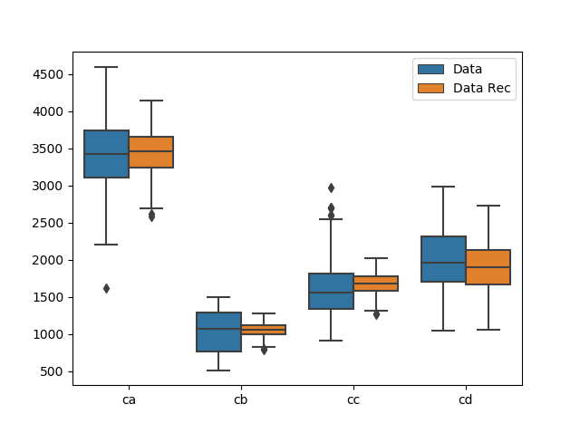
Grouped boxplot showing data before and after data reconciliation.

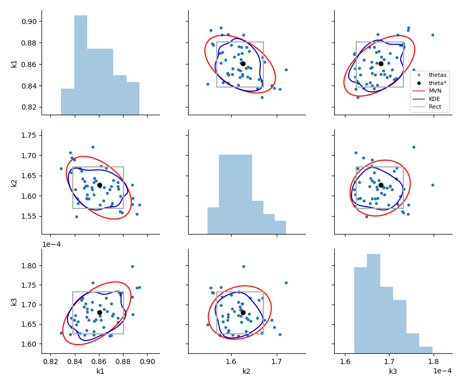
Pairwise bootstrap plot with rectangular, multivariate normal and kernel density estimation confidence region.

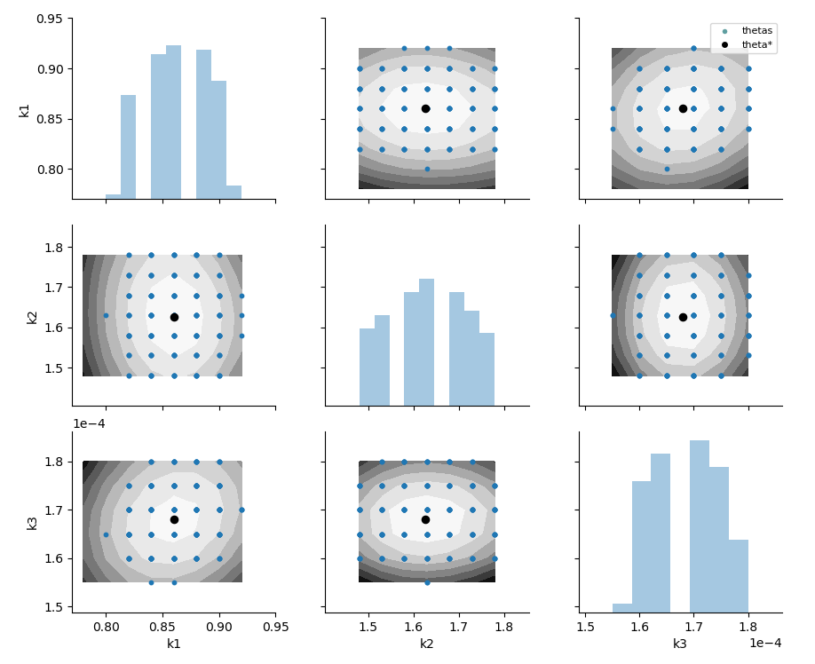
Pairwise likelihood ratio plot with contours of the objective and points that lie within an alpha confidence region.

Examples

Examples can be found in pyomo/contrib/parmest/examples and include:

• Reactor design example [PyomoBookII]

• Semibatch example [SemiBatch]

• Rooney Biegler example [RooneyBiegler]

Each example includes a Python file that contains the Pyomo model and a Python file to run parameter estimation.

Additional use cases include:

• Data reconciliation (reactor design example)

• Parameter estimation using data with duplicate sensors and time-series data (reactor design example)

• Parameter estimation using mpi4py, the example saves results to a file for later analysis/graphics (semibatch example)

The example below uses the reactor design example. The file reactor_design.py includes a function which returns an populated instance of the Pyomo model. Note that the model is defined to maximize cb and that k1, k2, and k3 are fixed. The _main_ program is included for easy testing of the model declaration.

#  ___________________________________________________________________________
#
#  Pyomo: Python Optimization Modeling Objects
#  Copyright (c) 2008-2024
#  National Technology and Engineering Solutions of Sandia, LLC
#  Under the terms of Contract DE-NA0003525 with National Technology and
#  Engineering Solutions of Sandia, LLC, the U.S. Government retains certain
#  rights in this software.
#  This software is distributed under the 3-clause BSD License.
#  ___________________________________________________________________________
"""
Continuously stirred tank reactor model, based on
pyomo/examples/doc/pyomobook/nonlinear-ch/react_design/ReactorDesign.py
"""

from pyomo.common.dependencies import pandas as pd
import pyomo.environ as pyo
import pyomo.contrib.parmest.parmest as parmest
from pyomo.contrib.parmest.experiment import Experiment


def reactor_design_model():

    # Create the concrete model
    model = pyo.ConcreteModel()

    # Rate constants
    model.k1 = pyo.Param(
        initialize=5.0 / 6.0, within=pyo.PositiveReals, mutable=True
    )  # min^-1
    model.k2 = pyo.Param(
        initialize=5.0 / 3.0, within=pyo.PositiveReals, mutable=True
    )  # min^-1
    model.k3 = pyo.Param(
        initialize=1.0 / 6000.0, within=pyo.PositiveReals, mutable=True
    )  # m^3/(gmol min)

    # Inlet concentration of A, gmol/m^3
    model.caf = pyo.Param(initialize=10000, within=pyo.PositiveReals, mutable=True)

    # Space velocity (flowrate/volume)
    model.sv = pyo.Param(initialize=1.0, within=pyo.PositiveReals, mutable=True)

    # Outlet concentration of each component
    model.ca = pyo.Var(initialize=5000.0, within=pyo.PositiveReals)
    model.cb = pyo.Var(initialize=2000.0, within=pyo.PositiveReals)
    model.cc = pyo.Var(initialize=2000.0, within=pyo.PositiveReals)
    model.cd = pyo.Var(initialize=1000.0, within=pyo.PositiveReals)

    # Objective
    model.obj = pyo.Objective(expr=model.cb, sense=pyo.maximize)

    # Constraints
    model.ca_bal = pyo.Constraint(
        expr=(
            0
            == model.sv * model.caf
            - model.sv * model.ca
            - model.k1 * model.ca
            - 2.0 * model.k3 * model.ca**2.0
        )
    )

    model.cb_bal = pyo.Constraint(
        expr=(0 == -model.sv * model.cb + model.k1 * model.ca - model.k2 * model.cb)
    )

    model.cc_bal = pyo.Constraint(
        expr=(0 == -model.sv * model.cc + model.k2 * model.cb)
    )

    model.cd_bal = pyo.Constraint(
        expr=(0 == -model.sv * model.cd + model.k3 * model.ca**2.0)
    )

    return model


class ReactorDesignExperiment(Experiment):

    def __init__(self, data, experiment_number):
        self.data = data
        self.experiment_number = experiment_number
        self.data_i = data.loc[experiment_number, :]
        self.model = None

    def create_model(self):
        self.model = m = reactor_design_model()
        return m

    def finalize_model(self):
        m = self.model

        # Experiment inputs values
        m.sv = self.data_i['sv']
        m.caf = self.data_i['caf']

        # Experiment output values
        m.ca = self.data_i['ca']
        m.cb = self.data_i['cb']
        m.cc = self.data_i['cc']
        m.cd = self.data_i['cd']

        return m

    def label_model(self):
        m = self.model

        m.experiment_outputs = pyo.Suffix(direction=pyo.Suffix.LOCAL)
        m.experiment_outputs.update(
            [
                (m.ca, self.data_i['ca']),
                (m.cb, self.data_i['cb']),
                (m.cc, self.data_i['cc']),
                (m.cd, self.data_i['cd']),
            ]
        )

        m.unknown_parameters = pyo.Suffix(direction=pyo.Suffix.LOCAL)
        m.unknown_parameters.update(
            (k, pyo.ComponentUID(k)) for k in [m.k1, m.k2, m.k3]
        )

        return m

    def get_labeled_model(self):
        m = self.create_model()
        m = self.finalize_model()
        m = self.label_model()

        return m


def main():

    # For a range of sv values, return ca, cb, cc, and cd
    results = []
    sv_values = [1.0 + v * 0.05 for v in range(1, 20)]
    caf = 10000
    for sv in sv_values:

        # make model
        model = reactor_design_model()

        # add caf, sv
        model.caf = caf
        model.sv = sv

        # solve model
        solver = pyo.SolverFactory("ipopt")
        solver.solve(model)

        # save results
        results.append([sv, caf, model.ca(), model.cb(), model.cc(), model.cd()])

    results = pd.DataFrame(results, columns=["sv", "caf", "ca", "cb", "cc", "cd"])
    print(results)


if __name__ == "__main__":
    main()

The file parameter_estimation_example.py uses parmest to estimate values of k1, k2, and k3 by minimizing the sum of squared error between model and observed values of ca, cb, cc, and cd. Additional example files use parmest to run parameter estimation with bootstrap resampling and perform a likelihood ratio test over a range of theta values.

#  ___________________________________________________________________________
#
#  Pyomo: Python Optimization Modeling Objects
#  Copyright (c) 2008-2024
#  National Technology and Engineering Solutions of Sandia, LLC
#  Under the terms of Contract DE-NA0003525 with National Technology and
#  Engineering Solutions of Sandia, LLC, the U.S. Government retains certain
#  rights in this software.
#  This software is distributed under the 3-clause BSD License.
#  ___________________________________________________________________________

from pyomo.common.dependencies import pandas as pd
from os.path import join, abspath, dirname
import pyomo.contrib.parmest.parmest as parmest
from pyomo.contrib.parmest.examples.reactor_design.reactor_design import (
    ReactorDesignExperiment,
)


def main():

    # Read in data
    file_dirname = dirname(abspath(str(__file__)))
    file_name = abspath(join(file_dirname, "reactor_data.csv"))
    data = pd.read_csv(file_name)

    # Create an experiment list
    exp_list = []
    for i in range(data.shape[0]):
        exp_list.append(ReactorDesignExperiment(data, i))

    # View one model
    # exp0_model = exp_list[0].get_labeled_model()
    # exp0_model.pprint()

    pest = parmest.Estimator(exp_list, obj_function='SSE')

    # Parameter estimation with covariance
    obj, theta, cov = pest.theta_est(calc_cov=True, cov_n=17)
    print(obj)
    print(theta)


if __name__ == "__main__":
    main()

The semibatch and Rooney Biegler examples are defined in a similar manner.

Parallel Implementation

Parallel implementation in parmest is preliminary. To run parmest in parallel, you need the mpi4py Python package and a compatible MPI installation. If you do NOT have mpi4py or a MPI installation, parmest still works (you should not get MPI import errors).

For example, the following command can be used to run the semibatch model in parallel:

mpiexec -n 4 python parallel_example.py

The file parallel_example.py is shown below. Results are saved to file for later analysis.

#  ___________________________________________________________________________
#
#  Pyomo: Python Optimization Modeling Objects
#  Copyright (c) 2008-2024
#  National Technology and Engineering Solutions of Sandia, LLC
#  Under the terms of Contract DE-NA0003525 with National Technology and
#  Engineering Solutions of Sandia, LLC, the U.S. Government retains certain
#  rights in this software.
#  This software is distributed under the 3-clause BSD License.
#  ___________________________________________________________________________

"""
The following script can be used to run semibatch parameter estimation in 
parallel and save results to files for later analysis and graphics.
Example command: mpiexec -n 4 python parallel_example.py
"""
from pyomo.common.dependencies import numpy as np, pandas as pd
from itertools import product
from os.path import join, abspath, dirname
import pyomo.contrib.parmest.parmest as parmest
from pyomo.contrib.parmest.examples.semibatch.semibatch import generate_model


def main():
    # Vars to estimate
    theta_names = ['k1', 'k2', 'E1', 'E2']

    # Data, list of json file names
    data = []
    file_dirname = dirname(abspath(str(__file__)))
    for exp_num in range(10):
        file_name = abspath(join(file_dirname, 'exp' + str(exp_num + 1) + '.out'))
        data.append(file_name)

    # Note, the model already includes a 'SecondStageCost' expression
    # for sum of squared error that will be used in parameter estimation

    pest = parmest.Estimator(generate_model, data, theta_names)

    ### Parameter estimation with bootstrap resampling
    bootstrap_theta = pest.theta_est_bootstrap(100)
    bootstrap_theta.to_csv('bootstrap_theta.csv')

    ### Compute objective at theta for likelihood ratio test
    k1 = np.arange(4, 24, 3)
    k2 = np.arange(40, 160, 40)
    E1 = np.arange(29000, 32000, 500)
    E2 = np.arange(38000, 42000, 500)
    theta_vals = pd.DataFrame(list(product(k1, k2, E1, E2)), columns=theta_names)

    obj_at_theta = pest.objective_at_theta(theta_vals)
    obj_at_theta.to_csv('obj_at_theta.csv')


if __name__ == "__main__":
    main()

Installation

The mpi4py Python package should be installed using conda. The following installation instructions were tested on a Mac with Python 3.5.

Create a conda environment and install mpi4py using the following commands:

conda create -n parmest-parallel python=3.5
source activate parmest-parallel
conda install -c conda-forge mpi4py

This should install libgfortran, mpi, mpi4py, and openmpi.

To verify proper installation, create a Python file with the following:

from mpi4py import MPI
import time
comm = MPI.COMM_WORLD
rank = comm.Get_rank()
print('Rank = ',rank)
time.sleep(10)

Save the file as test_mpi.py and run the following command:

time mpiexec -n 4 python test_mpi.py
time python test_mpi.py

The first one should be faster and should start 4 instances of Python.

API

parmest

class pyomo.contrib.parmest.parmest.Estimator(experiment_list, obj_function=None, tee=False, diagnostic_mode=False, solver_options=None)

Bases: object

Parameter estimation class

Parameters:

• experiment_list (list of Experiments) – A list of experiment objects which creates one labeled model for each experiment

• obj_function (string or function (optional)) – Built in objective (currently only “SSE”) or custom function used to formulate parameter estimation objective. If no function is specified, the model is used “as is” and should be defined with a “FirstStageCost” and “SecondStageCost” expression that are used to build an objective. Default is None.

• tee (bool, optional) – If True, print the solver output to the screen. Default is False.

• diagnostic_mode (bool, optional) – If True, print diagnostics from the solver. Default is False.

• solver_options (dict, optional) – Provides options to the solver (also the name of an attribute). Default is None.

confidence_region_test(theta_values, distribution, alphas, test_theta_values=None)

Confidence region test to determine if theta values are within a rectangular, multivariate normal, or Gaussian kernel density distribution for a range of alpha values

Parameters:

• theta_values (pd.DataFrame, columns = theta_names) – Theta values used to generate a confidence region (generally returned by theta_est_bootstrap)

• distribution (string) – Statistical distribution used to define a confidence region, options = ‘MVN’ for multivariate_normal, ‘KDE’ for gaussian_kde, and ‘Rect’ for rectangular.

• alphas (list) – List of alpha values used to determine if theta values are inside or outside the region.

• test_theta_values (pd.Series or pd.DataFrame, keys/columns = theta_names, optional) – Additional theta values that are compared to the confidence region to determine if they are inside or outside.

Returns:

• training_results (pd.DataFrame) – Theta value used to generate the confidence region along with True (inside) or False (outside) for each alpha

• test_results (pd.DataFrame) – If test_theta_values is not None, returns test theta value along with True (inside) or False (outside) for each alpha

leaveNout_bootstrap_test(lNo, lNo_samples, bootstrap_samples, distribution, alphas, seed=None)

Leave-N-out bootstrap test to compare theta values where N data points are left out to a bootstrap analysis using the remaining data, results indicate if theta is within a confidence region determined by the bootstrap analysis

Parameters:

• lNo (int) – Number of data points to leave out for parameter estimation

• lNo_samples (int) – Leave-N-out sample size. If lNo_samples=None, the maximum number of combinations will be used

• bootstrap_samples (int:) – Bootstrap sample size

• distribution (string) – Statistical distribution used to define a confidence region, options = ‘MVN’ for multivariate_normal, ‘KDE’ for gaussian_kde, and ‘Rect’ for rectangular.

• alphas (list) – List of alpha values used to determine if theta values are inside or outside the region.

• seed (int or None, optional) – Random seed

Returns:

• List of tuples with one entry per lNo_sample

• * The first item in each tuple is the list of N samples that are left – out.

• * The second item in each tuple is a DataFrame of theta estimated using – the N samples.

• * The third item in each tuple is a DataFrame containing results from – the bootstrap analysis using the remaining samples.

• For each DataFrame a column is added for each value of alpha which

• indicates if the theta estimate is in (True) or out (False) of the

• alpha region for a given distribution (based on the bootstrap results)

likelihood_ratio_test(obj_at_theta, obj_value, alphas, return_thresholds=False)

Likelihood ratio test to identify theta values within a confidence region using the \(\chi^2\) distribution

Parameters:

• obj_at_theta (pd.DataFrame, columns = theta_names + 'obj') – Objective values for each theta value (returned by objective_at_theta)

• obj_value (int or float) – Objective value from parameter estimation using all data

• alphas (list) – List of alpha values to use in the chi2 test

• return_thresholds (bool, optional) – Return the threshold value for each alpha. Default is False.

Returns:

• LR (pd.DataFrame) – Objective values for each theta value along with True or False for each alpha

• thresholds (pd.Series) – If return_threshold = True, the thresholds are also returned.

objective_at_theta(theta_values=None, initialize_parmest_model=False)

Objective value for each theta

Parameters:

• theta_values (pd.DataFrame, columns=theta_names) – Values of theta used to compute the objective

• initialize_parmest_model (boolean) – If True: Solve square problem instance, build extensive form of the model for parameter estimation, and set flag model_initialized to True. Default is False.

Returns:

obj_at_theta – Objective value for each theta (infeasible solutions are omitted).

Return type:

pd.DataFrame

theta_est(solver='ef_ipopt', return_values=[], calc_cov=False, cov_n=None)

Parameter estimation using all scenarios in the data

Parameters:

• solver (string, optional) – Currently only “ef_ipopt” is supported. Default is “ef_ipopt”.

• return_values (list, optional) – List of Variable names, used to return values from the model for data reconciliation

• calc_cov (boolean, optional) – If True, calculate and return the covariance matrix (only for “ef_ipopt” solver). Default is False.

• cov_n (int, optional) – If calc_cov=True, then the user needs to supply the number of datapoints that are used in the objective function.

Returns:

• objectiveval (float) – The objective function value

• thetavals (pd.Series) – Estimated values for theta

• variable values (pd.DataFrame) – Variable values for each variable name in return_values (only for solver=’ef_ipopt’)

• cov (pd.DataFrame) – Covariance matrix of the fitted parameters (only for solver=’ef_ipopt’)

theta_est_bootstrap(bootstrap_samples, samplesize=None, replacement=True, seed=None, return_samples=False)

Parameter estimation using bootstrap resampling of the data

Parameters:

• bootstrap_samples (int) – Number of bootstrap samples to draw from the data

• samplesize (int or None, optional) – Size of each bootstrap sample. If samplesize=None, samplesize will be set to the number of samples in the data

• replacement (bool, optional) – Sample with or without replacement. Default is True.

• seed (int or None, optional) – Random seed

• return_samples (bool, optional) – Return a list of sample numbers used in each bootstrap estimation. Default is False.

Returns:

bootstrap_theta – Theta values for each sample and (if return_samples = True) the sample numbers used in each estimation

Return type:

pd.DataFrame

theta_est_leaveNout(lNo, lNo_samples=None, seed=None, return_samples=False)

Parameter estimation where N data points are left out of each sample

Parameters:

• lNo (int) – Number of data points to leave out for parameter estimation

• lNo_samples (int) – Number of leave-N-out samples. If lNo_samples=None, the maximum number of combinations will be used

• seed (int or None, optional) – Random seed

• return_samples (bool, optional) – Return a list of sample numbers that were left out. Default is False.

Returns:

lNo_theta – Theta values for each sample and (if return_samples = True) the sample numbers left out of each estimation

Return type:

pd.DataFrame

pyomo.contrib.parmest.parmest.SSE(model)

Sum of squared error between experiment_output model and data values

pyomo.contrib.parmest.parmest.ef_nonants(ef)

pyomo.contrib.parmest.parmest.group_data(data, groupby_column_name, use_mean=None)

DEPRECATED.

Group data by scenario

data: DataFrame

Data

groupby_column_name: strings

Name of data column which contains scenario numbers

use_mean: list of column names or None, optional

Name of data columns which should be reduced to a single value per scenario by taking the mean

grouped_data: list of dictionaries

Grouped data

Deprecated since version 6.7.2: This function (group_data) has been deprecated and may be removed in a future release.

scenariocreator

class pyomo.contrib.parmest.scenariocreator.ParmestScen(name, ThetaVals, probability)

Bases: object

A little container for scenarios; the Args are the attributes.

Parameters:

• name (str) – name for reporting; might be “”

• ThetaVals (dict) – ThetaVals[name]=val

• probability (float) – probability of occurrence “near” these ThetaVals

class pyomo.contrib.parmest.scenariocreator.ScenarioCreator(pest, solvername)

Bases: object

Create scenarios from parmest.

Parameters:

• pest (Estimator) – the parmest object

• solvername (str) – name of the solver (e.g. “ipopt”)

ScenariosFromBootstrap(addtoSet, numtomake, seed=None)

Creates new self.Scenarios list using the experiments only.

Parameters:

• addtoSet (ScenarioSet) – the scenarios will be added to this set

• numtomake (int) – number of scenarios to create

ScenariosFromExperiments(addtoSet)

Creates new self.Scenarios list using the experiments only.

Parameters:

addtoSet (ScenarioSet) – the scenarios will be added to this set

Returns:

a ScenarioSet

class pyomo.contrib.parmest.scenariocreator.ScenarioSet(name)

Bases: object

Class to hold scenario sets

Args: name (str): name of the set (might be “”)

ScenarioNumber(scennum)

Returns the scenario with the given, zero-based number

ScensIterator()

Usage: for scenario in ScensIterator()

addone(scen)

Add a scenario to the set

Parameters:

scen (ParmestScen) – the scenario to add

append_bootstrap(bootstrap_theta)

Append a bootstrap theta df to the scenario set; equally likely

Parameters:

bootstrap_theta (dataframe) – created by the bootstrap

Note: this can be cleaned up a lot with the list becomes a df,

which is why I put it in the ScenarioSet class.

write_csv(filename)

write a csv file with the scenarios in the set

Parameters:

filename (str) – full path and full name of file

graphics

pyomo.contrib.parmest.graphics.fit_kde_dist(theta_values)

Fit a Gaussian kernel-density distribution to theta values

Parameters:

theta_values (DataFrame) – Theta values, columns = variable names

Return type:

scipy.stats.gaussian_kde distribution

pyomo.contrib.parmest.graphics.fit_mvn_dist(theta_values)

Fit a multivariate normal distribution to theta values

Parameters:

theta_values (DataFrame) – Theta values, columns = variable names

Return type:

scipy.stats.multivariate_normal distribution

pyomo.contrib.parmest.graphics.fit_rect_dist(theta_values, alpha)

Fit an alpha-level rectangular distribution to theta values

Parameters:

• theta_values (DataFrame) – Theta values, columns = variable names

• alpha (float, optional) – Confidence interval value

Return type:

tuple containing lower bound and upper bound for each variable

pyomo.contrib.parmest.graphics.grouped_boxplot(data1, data2, normalize=False, group_names=['data1', 'data2'], filename=None)

Plot a grouped boxplot to compare two datasets

The datasets can be normalized by the median and standard deviation of data1.

Parameters:

• data1 (DataFrame) – Data set, columns = variable names

• data2 (DataFrame) – Data set, columns = variable names

• normalize (bool, optional) – Normalize both datasets by the median and standard deviation of data1

• group_names (list, optional) – Names used in the legend

• filename (string, optional) – Filename used to save the figure

pyomo.contrib.parmest.graphics.grouped_violinplot(data1, data2, normalize=False, group_names=['data1', 'data2'], filename=None)

Plot a grouped violinplot to compare two datasets

The datasets can be normalized by the median and standard deviation of data1.

Parameters:

• data1 (DataFrame) – Data set, columns = variable names

• data2 (DataFrame) – Data set, columns = variable names

• normalize (bool, optional) – Normalize both datasets by the median and standard deviation of data1

• group_names (list, optional) – Names used in the legend

• filename (string, optional) – Filename used to save the figure

pyomo.contrib.parmest.graphics.pairwise_plot(theta_values, theta_star=None, alpha=None, distributions=[], axis_limits=None, title=None, add_obj_contour=True, add_legend=True, filename=None)

Plot pairwise relationship for theta values, and optionally alpha-level confidence intervals and objective value contours

Parameters:

• theta_values (DataFrame or tuple) –

  • If theta_values is a DataFrame, then it contains one column for each theta variable and (optionally) an objective value column (‘obj’) and columns that contains Boolean results from confidence interval tests (labeled using the alpha value). Each row is a sample.

    • Theta variables can be computed from theta_est_bootstrap, theta_est_leaveNout, and leaveNout_bootstrap_test.

    • The objective value can be computed using the likelihood_ratio_test.

    • Results from confidence interval tests can be computed using the leaveNout_bootstrap_test, likelihood_ratio_test, and confidence_region_test.

  • If theta_values is a tuple, then it contains a mean, covariance, and number of samples (mean, cov, n) where mean is a dictionary or Series (indexed by variable name), covariance is a DataFrame (indexed by variable name, one column per variable name), and n is an integer. The mean and covariance are used to create a multivariate normal sample of n theta values. The covariance can be computed using theta_est(calc_cov=True).

• theta_star (dict or Series, optional) – Estimated value of theta. The dictionary or Series is indexed by variable name. Theta_star is used to slice higher dimensional contour intervals in 2D

• alpha (float, optional) – Confidence interval value, if an alpha value is given and the distributions list is empty, the data will be filtered by True/False values using the column name whose value equals alpha (see results from leaveNout_bootstrap_test, likelihood_ratio_test, and confidence_region_test)

• distributions (list of strings, optional) – Statistical distribution used to define a confidence region, options = ‘MVN’ for multivariate_normal, ‘KDE’ for gaussian_kde, and ‘Rect’ for rectangular. Confidence interval is a 2D slice, using linear interpolation at theta_star.

• axis_limits (dict, optional) – Axis limits in the format {variable: [min, max]}

• title (string, optional) – Plot title

• add_obj_contour (bool, optional) – Add a contour plot using the column ‘obj’ in theta_values. Contour plot is a 2D slice, using linear interpolation at theta_star.

• add_legend (bool, optional) – Add a legend to the plot

• filename (string, optional) – Filename used to save the figure

Indices and Tables

• Index

• Module Index

• Search Page

PyNumero

PyNumero is a package for developing parallel algorithms for nonlinear programs (NLPs). This documentation provides a brief introduction to PyNumero. For more details, see the API documentation (PyNumero API).

PyNumero Installation

PyNumero is a module within Pyomo. Therefore, Pyomo must be installed to use PyNumero. PyNumero also has some extensions that need built. There are many ways to build the PyNumero extensions. Common use cases are listed below. However, more information can always be found at https://github.com/Pyomo/pyomo/blob/main/pyomo/contrib/pynumero/build.py and https://github.com/Pyomo/pyomo/blob/main/pyomo/contrib/pynumero/src/CMakeLists.txt.

Note that you will need a C++ compiler and CMake installed to build the PyNumero libraries.

Method 1

One way to build PyNumero extensions is with the pyomo download-extensions and build-extensions subcommands. Note that this approach will build PyNumero without support for the HSL linear solvers.

pyomo download-extensions
pyomo build-extensions

Method 2

If you want PyNumero support for the HSL solvers and you have an IPOPT compilation for your machine, you can build PyNumero using the build script

python -m pyomo.contrib.pynumero.build -DBUILD_ASL=ON -DBUILD_MA27=ON -DIPOPT_DIR=<path/to/ipopt/build/>

Method 3

You can build the PyNumero libraries from source using cmake. This generally works best when building from a source distribution of Pyomo. Assuming that you are starting in the root of the Pyomo source distribution, you can follow the normal CMake build process

mkdir build
cd build
ccmake ../pyomo/contrib/pynumero/src
make
make install

10 Minutes to PyNumero

NLP Interfaces

Below are examples of using PyNumero’s interfaces to ASL for function and derivative evaluation. More information can be found in the API documentation (PyNumero API).

Relevant imports

>>> import pyomo.environ as pe
>>> from pyomo.contrib.pynumero.interfaces.pyomo_nlp import PyomoNLP
>>> import numpy as np

Create a Pyomo model

>>> m = pe.ConcreteModel()
>>> m.x = pe.Var(bounds=(-5, None))
>>> m.y = pe.Var(initialize=2.5)
>>> m.obj = pe.Objective(expr=m.x**2 + m.y**2)
>>> m.c1 = pe.Constraint(expr=m.y == (m.x - 1)**2)
>>> m.c2 = pe.Constraint(expr=m.y >= pe.exp(m.x))

Create a pyomo.contrib.pynumero.interfaces.pyomo_nlp.PyomoNLP instance

>>> nlp = PyomoNLP(m)

Get values of primals and duals

>>> nlp.get_primals()
array([0. , 2.5])
>>> nlp.get_duals()
array([0., 0.])

Get variable and constraint bounds

>>> nlp.primals_lb()
array([ -5., -inf])
>>> nlp.primals_ub()
array([inf, inf])
>>> nlp.constraints_lb()
array([  0., -inf])
>>> nlp.constraints_ub()
array([0., 0.])

Objective and constraint evaluations

>>> nlp.evaluate_objective()
6.25
>>> nlp.evaluate_constraints()
array([ 1.5, -1.5])

Derivative evaluations

>>> nlp.evaluate_grad_objective()
array([0., 5.])
>>> nlp.evaluate_jacobian()  
<2x2 sparse matrix of type '<class 'numpy.float64'>'
    with 4 stored elements in COOrdinate format>
>>> nlp.evaluate_jacobian().toarray()
array([[ 2.,  1.],
       [ 1., -1.]])
>>> nlp.evaluate_hessian_lag().toarray()
array([[2., 0.],
       [0., 2.]])

Set values of primals and duals

>>> nlp.set_primals(np.array([0, 1]))
>>> nlp.evaluate_constraints()
array([0., 0.])
>>> nlp.set_duals(np.array([-2/3, 4/3]))
>>> nlp.evaluate_grad_objective() + nlp.evaluate_jacobian().transpose() * nlp.get_duals()
array([0., 0.])

Equality and inequality constraints separately

>>> nlp.evaluate_eq_constraints()
array([0.])
>>> nlp.evaluate_jacobian_eq().toarray()
array([[2., 1.]])
>>> nlp.evaluate_ineq_constraints()
array([0.])
>>> nlp.evaluate_jacobian_ineq().toarray()
array([[ 1., -1.]])
>>> nlp.get_duals_eq()
array([-0.66666667])
>>> nlp.get_duals_ineq()
array([1.33333333])

Linear Solver Interfaces

PyNumero’s interfaces to linear solvers are very thin wrappers, and, hence, are rather low-level. It is relatively easy to wrap these again for specific applications. For example, see the linear solver interfaces in https://github.com/Pyomo/pyomo/tree/main/pyomo/contrib/interior_point/linalg, which wrap PyNumero’s linear solver interfaces.

The motivation to keep PyNumero’s interfaces as such thin wrappers is that different linear solvers serve different purposes. For example, HSL’s MA27 can factorize symmetric indefinite matrices, while MUMPS can factorize unsymmetric, symmetric positive definite, or general symmetric matrices. PyNumero seeks to be independent of the application, giving more flexibility to algorithm developers.

Interface to MA27

>>> import numpy as np
>>> from scipy.sparse import coo_matrix
>>> from scipy.sparse import tril
>>> from pyomo.contrib.pynumero.linalg.ma27_interface import MA27
>>> row = np.array([0, 1, 0, 1, 0, 1, 2, 3, 3, 4, 4, 4])
>>> col = np.array([0, 1, 3, 3, 4, 4, 4, 0, 1, 0, 1, 2])
>>> data = np.array([1.67025575, 2, -1.64872127,  1, -1, -1, -1, -1.64872127, 1, -1, -1, -1])
>>> A = coo_matrix((data, (row, col)), shape=(5,5))
>>> A.toarray()
array([[ 1.67025575,  0.        ,  0.        , -1.64872127, -1.        ],
       [ 0.        ,  2.        ,  0.        ,  1.        , -1.        ],
       [ 0.        ,  0.        ,  0.        ,  0.        , -1.        ],
       [-1.64872127,  1.        ,  0.        ,  0.        ,  0.        ],
       [-1.        , -1.        , -1.        ,  0.        ,  0.        ]])
>>> rhs = np.array([-0.67025575, -1.2,  0.1,  1.14872127,  1.25])
>>> solver = MA27()
>>> solver.set_cntl(1, 1e-6)  # set the pivot tolerance
>>> status = solver.do_symbolic_factorization(A)
>>> status = solver.do_numeric_factorization(A)
>>> x, status = solver.do_back_solve(rhs)
>>> np.max(np.abs(A*x - rhs)) <= 1e-15
True

Interface to MUMPS

>>> import numpy as np
>>> from scipy.sparse import coo_matrix
>>> from scipy.sparse import tril
>>> from pyomo.contrib.pynumero.linalg.mumps_interface import MumpsCentralizedAssembledLinearSolver
>>> row = np.array([0, 1, 0, 1, 0, 1, 2, 3, 3, 4, 4, 4])
>>> col = np.array([0, 1, 3, 3, 4, 4, 4, 0, 1, 0, 1, 2])
>>> data = np.array([1.67025575, 2, -1.64872127,  1, -1, -1, -1, -1.64872127, 1, -1, -1, -1])
>>> A = coo_matrix((data, (row, col)), shape=(5,5))
>>> A.toarray()
array([[ 1.67025575,  0.        ,  0.        , -1.64872127, -1.        ],
       [ 0.        ,  2.        ,  0.        ,  1.        , -1.        ],
       [ 0.        ,  0.        ,  0.        ,  0.        , -1.        ],
       [-1.64872127,  1.        ,  0.        ,  0.        ,  0.        ],
       [-1.        , -1.        , -1.        ,  0.        ,  0.        ]])
>>> rhs = np.array([-0.67025575, -1.2,  0.1,  1.14872127,  1.25])
>>> solver = MumpsCentralizedAssembledLinearSolver(sym=2, par=1, comm=None)  # symmetric matrix; solve in serial
>>> solver.do_symbolic_factorization(A)
>>> solver.do_numeric_factorization(A)
>>> x = solver.do_back_solve(rhs)
>>> np.max(np.abs(A*x - rhs)) <= 1e-15
True

Of course, SciPy solvers can also be used. See SciPy documentation for details.

Block Vectors and Matrices

Block vectors and matrices (BlockVector and BlockMatrix) provide a mechanism to perform linear algebra operations with very structured matrices and vectors.

When a BlockVector or BlockMatrix is constructed, the number of blocks must be specified.

>>> import numpy as np
>>> from scipy.sparse import coo_matrix
>>> from pyomo.contrib.pynumero.sparse import BlockVector, BlockMatrix
>>> v = BlockVector(3)
>>> m = BlockMatrix(3, 3)

Setting blocks:

>>> v.set_block(0, np.array([-0.67025575, -1.2]))
>>> v.set_block(1, np.array([0.1, 1.14872127]))
>>> v.set_block(2, np.array([1.25]))
>>> v.flatten()
array([-0.67025575, -1.2       ,  0.1       ,  1.14872127,  1.25      ])

The flatten method converts the BlockVector into a NumPy array.

>>> m.set_block(0, 0, coo_matrix(np.array([[1.67025575, 0], [0, 2]])))
>>> m.set_block(0, 1, coo_matrix(np.array([[0, -1.64872127], [0, 1]])))
>>> m.set_block(0, 2, coo_matrix(np.array([[-1.0], [-1]])))
>>> m.set_block(1, 0, coo_matrix(np.array([[0, -1.64872127], [0, 1]])).transpose())
>>> m.set_block(1, 2, coo_matrix(np.array([[-1.0], [0]])))
>>> m.set_block(2, 0, coo_matrix(np.array([[-1.0], [-1]])).transpose())
>>> m.set_block(2, 1, coo_matrix(np.array([[-1.0], [0]])).transpose())
>>> m.tocoo().toarray()
array([[ 1.67025575,  0.        ,  0.        , -1.64872127, -1.        ],
       [ 0.        ,  2.        ,  0.        ,  1.        , -1.        ],
       [ 0.        ,  0.        ,  0.        ,  0.        , -1.        ],
       [-1.64872127,  1.        ,  0.        ,  0.        ,  0.        ],
       [-1.        , -1.        , -1.        ,  0.        ,  0.        ]])

The tocoo method converts the BlockMatrix to a SciPy sparse coo_matrix.

Once the dimensions of a block have been set, they cannot be changed:

>>> v.set_block(0, np.ones(3))
Traceback (most recent call last):
  ...
ValueError: Incompatible dimensions for block 0; got 3; expected 2

Properties:

>>> v.shape
(5,)
>>> v.size
5
>>> v.nblocks
3
>>> v.bshape
(3,)
>>> m.shape
(5, 5)
>>> m.bshape
(3, 3)
>>> m.nnz
12

Much of the BlockVector API matches that of NumPy arrays:

>>> v.sum()
0.62846552
>>> v.max()
1.25
>>> np.abs(v).flatten()
array([0.67025575, 1.2       , 0.1       , 1.14872127, 1.25      ])
>>> (2*v).flatten()
array([-1.3405115 , -2.4       ,  0.2       ,  2.29744254,  2.5       ])
>>> (v + v).flatten()
array([-1.3405115 , -2.4       ,  0.2       ,  2.29744254,  2.5       ])
>>> v.dot(v)
4.781303326558476

Similarly, BlockMatrix behaves very similarly to SciPy sparse matrices:

>>> (2*m).tocoo().toarray()
array([[ 3.3405115 ,  0.        ,  0.        , -3.29744254, -2.        ],
       [ 0.        ,  4.        ,  0.        ,  2.        , -2.        ],
       [ 0.        ,  0.        ,  0.        ,  0.        , -2.        ],
       [-3.29744254,  2.        ,  0.        ,  0.        ,  0.        ],
       [-2.        , -2.        , -2.        ,  0.        ,  0.        ]])
>>> (m - m).tocoo().toarray()
array([[0., 0., 0., 0., 0.],
       [0., 0., 0., 0., 0.],
       [0., 0., 0., 0., 0.],
       [0., 0., 0., 0., 0.],
       [0., 0., 0., 0., 0.]])
>>> m * v
BlockVector(3,)
>>> (m * v).flatten()
array([-4.26341971, -2.50127873, -1.25      , -0.09493509,  1.77025575])

Accessing blocks

>>> v.get_block(1)
array([0.1       , 1.14872127])
>>> m.get_block(1, 0).toarray()
array([[ 0.        ,  0.        ],
       [-1.64872127,  1.        ]])

Empty blocks in a BlockMatrix return None:

>>> print(m.get_block(1, 1))
None

The dimensions of a blocks in a BlockMatrix can be set without setting a block:

>>> m2 = BlockMatrix(2, 2)
>>> m2.set_row_size(0, 5)
>>> m2.set_block(0, 0, m.get_block(0, 0))
Traceback (most recent call last):
  ...
ValueError: Incompatible row dimensions for row 0; got 2; expected 5.0

Note that operations on BlockVector and BlockMatrix cannot be performed until the dimensions are fully specified:

>>> v2 = BlockVector(3)
>>> v + v2
Traceback (most recent call last):
  ...
NotFullyDefinedBlockVectorError: Operation not allowed with None blocks.
>>> m2 = BlockMatrix(3, 3)
>>> m2 * 2
Traceback (most recent call last):
  ...
NotFullyDefinedBlockMatrixError: Operation not allowed with None rows. Specify at least one block in every row

The has_none property can be used to see if a BlockVector is fully specified. If has_none returns True, then there are None blocks, and the BlockVector is not fully specified.

>>> v.has_none
False
>>> v2.has_none
True

For BlockMatrix, use the has_undefined_row_sizes() and has_undefined_col_sizes() methods:

>>> m.has_undefined_row_sizes()
False
>>> m.has_undefined_col_sizes()
False
>>> m2.has_undefined_row_sizes()
True
>>> m2.has_undefined_col_sizes()
True

To efficiently iterate over non-empty blocks in a BlockMatrix, use the get_block_mask() method, which returns a 2-D array indicating where the non-empty blocks are:

>>> m.get_block_mask(copy=False)
array([[ True,  True,  True],
       [ True, False,  True],
       [ True,  True, False]])
>>> for i, j in zip(*np.nonzero(m.get_block_mask(copy=False))):
...     assert m.get_block(i, j) is not None

Copying data:

>>> v2 = v.copy()
>>> v2.flatten()
array([-0.67025575, -1.2       ,  0.1       ,  1.14872127,  1.25      ])
>>> v2 = v.copy_structure()
>>> v2.block_sizes()  
array([2, 2, 1])
>>> v2.copyfrom(v)
>>> v2.flatten()
array([-0.67025575, -1.2       ,  0.1       ,  1.14872127,  1.25      ])
>>> m2 = m.copy()
>>> (m - m2).tocoo().toarray()
array([[0., 0., 0., 0., 0.],
       [0., 0., 0., 0., 0.],
       [0., 0., 0., 0., 0.],
       [0., 0., 0., 0., 0.],
       [0., 0., 0., 0., 0.]])
>>> m2 = m.copy_structure()
>>> m2.has_undefined_row_sizes()
False
>>> m2.has_undefined_col_sizes()
False
>>> m2.copyfrom(m)
>>> (m - m2).tocoo().toarray()
array([[0., 0., 0., 0., 0.],
       [0., 0., 0., 0., 0.],
       [0., 0., 0., 0., 0.],
       [0., 0., 0., 0., 0.],
       [0., 0., 0., 0., 0.]])

Nested blocks:

>>> v2 = BlockVector(2)
>>> v2.set_block(0, v)
>>> v2.set_block(1, np.ones(2))
>>> v2.block_sizes()  
array([5, 2])
>>> v2.flatten()
array([-0.67025575, -1.2       ,  0.1       ,  1.14872127,  1.25      ,
        1.        ,  1.        ])
>>> v3 = v2.copy_structure()
>>> v3.fill(1)
>>> (v2 + v3).flatten()
array([ 0.32974425, -0.2       ,  1.1       ,  2.14872127,  2.25      ,
        2.        ,  2.        ])
>>> np.abs(v2).flatten()
array([0.67025575, 1.2       , 0.1       , 1.14872127, 1.25      ,
       1.        , 1.        ])
>>> v2.get_block(0)
BlockVector(3,)

Nested BlockMatrix applications work similarly.

For more information, see the API documentation (PyNumero API).

MPI-Based Block Vectors and Matrices

PyNumero’s MPI-based block vectors and matrices (MPIBlockVector and MPIBlockMatrix) behave very similarly to BlockVector and BlockMatrix. The primary difference is in construction. With MPIBlockVector and MPIBlockMatrix, each block is owned by either a single process/rank or all processes/ranks.

Consider the following example (in a file called “parallel_vector_ops.py”).

#  ___________________________________________________________________________
#
#  Pyomo: Python Optimization Modeling Objects
#  Copyright (c) 2008-2024
#  National Technology and Engineering Solutions of Sandia, LLC
#  Under the terms of Contract DE-NA0003525 with National Technology and
#  Engineering Solutions of Sandia, LLC, the U.S. Government retains certain
#  rights in this software.
#  This software is distributed under the 3-clause BSD License.
#  ___________________________________________________________________________

import numpy as np
from pyomo.common.dependencies import mpi4py
from pyomo.contrib.pynumero.sparse.mpi_block_vector import MPIBlockVector


def main():
    comm = mpi4py.MPI.COMM_WORLD
    rank = comm.Get_rank()

    owners = [2, 0, 1, -1]
    x = MPIBlockVector(4, rank_owner=owners, mpi_comm=comm)
    x.set_block(owners.index(rank), np.ones(3) * (rank + 1))
    x.set_block(3, np.array([1, 2, 3]))

    y = MPIBlockVector(4, rank_owner=owners, mpi_comm=comm)
    y.set_block(owners.index(rank), np.ones(3) * (rank + 1))
    y.set_block(3, np.array([1, 2, 3]))

    z1: MPIBlockVector = x + y  # add x and y
    z2 = x.dot(y)  # dot product
    z3 = np.abs(x).max()  # infinity norm

    z1_local = z1.make_local_copy()
    if rank == 0:
        print(z1_local.flatten())
        print(z2)
        print(z3)

    return z1_local, z2, z3


if __name__ == '__main__':
    main()

This example can be run with

mpirun -np 3 python -m mpi4py parallel_vector_ops.py

The output is

[6. 6. 6. 2. 2. 2. 4. 4. 4. 2. 4. 6.]
56.0
3

Note that the make_local_copy() method is not efficient and should only be used for debugging.

The -1 in owners means that the block at that index (index 3 in this example) is owned by all processes. The non-negative integer values indicate that the block at that index is owned by the process with rank equal to the value. In this example, rank 0 owns block 1, rank 1 owns block 2, and rank 2 owns block 0. Block 3 is owned by all ranks. Note that blocks should only be set if the process/rank owns that block.

The operations performed with MPIBlockVector are identical to the same operations performed with BlockVector (or even NumPy arrays), except that the operations are now performed in parallel.

MPIBlockMatrix construction is very similar. Consider the following example in a file called “parallel_matvec.py”.

#  ___________________________________________________________________________
#
#  Pyomo: Python Optimization Modeling Objects
#  Copyright (c) 2008-2024
#  National Technology and Engineering Solutions of Sandia, LLC
#  Under the terms of Contract DE-NA0003525 with National Technology and
#  Engineering Solutions of Sandia, LLC, the U.S. Government retains certain
#  rights in this software.
#  This software is distributed under the 3-clause BSD License.
#  ___________________________________________________________________________

import numpy as np
from pyomo.common.dependencies import mpi4py
from pyomo.contrib.pynumero.sparse.mpi_block_vector import MPIBlockVector
from pyomo.contrib.pynumero.sparse.mpi_block_matrix import MPIBlockMatrix
from scipy.sparse import random


def main():
    comm = mpi4py.MPI.COMM_WORLD
    rank = comm.Get_rank()

    owners = [0, 1, 2, -1]
    x = MPIBlockVector(4, rank_owner=owners, mpi_comm=comm)

    owners = np.array([[0, -1, -1, 0], [-1, 1, -1, 1], [-1, -1, 2, 2]])
    a = MPIBlockMatrix(3, 4, rank_ownership=owners, mpi_comm=comm)

    np.random.seed(0)
    x.set_block(3, np.random.uniform(-10, 10, size=10))

    np.random.seed(rank)
    x.set_block(rank, np.random.uniform(-10, 10, size=10))
    a.set_block(rank, rank, random(10, 10, density=0.1))
    a.set_block(rank, 3, random(10, 10, density=0.1))

    b = a * x  # parallel matrix-vector dot product

    # check the answer
    local_x = x.make_local_copy().flatten()
    local_a = a.to_local_array()
    local_b = b.make_local_copy().flatten()

    err = np.abs(local_a.dot(local_x) - local_b).max()

    if rank == 0:
        print('error: ', err)

    return err


if __name__ == '__main__':
    main()

Which can be run with

mpirun -np 3 python -m mpi4py parallel_matvec.py

The output is

error:  4.440892098500626e-16

The most difficult part of using MPIBlockVector and MPIBlockMatrix is determining the best structure and rank ownership to maximize parallel efficiency.

Other examples may be found at https://github.com/Pyomo/pyomo/tree/main/pyomo/contrib/pynumero/examples.

PyNumero API

PyNumero Block Linear Algebra

BlockVector

Methods specific to pyomo.contrib.pynumero.sparse.block_vector.BlockVector:

• set_block()

• get_block()

• block_sizes()

• get_block_size()

• is_block_defined()

• copyfrom()

• copyto()

• copy_structure()

• set_blocks()

• pprint()

Attributes specific to pyomo.contrib.pynumero.sparse.block_vector.BlockVector:

• nblocks

• bshape

• has_none

NumPy compatible methods:

• numpy.ndarray.dot()

• numpy.ndarray.sum()

• numpy.ndarray.all()

• numpy.ndarray.any()

• numpy.ndarray.max()

• numpy.ndarray.astype()

• numpy.ndarray.clip()

• numpy.ndarray.compress()

• numpy.ndarray.conj()

• numpy.ndarray.conjugate()

• numpy.ndarray.nonzero()

• numpy.ndarray.ptp()

• numpy.ndarray.round()

• numpy.ndarray.std()

• numpy.ndarray.var()

• numpy.ndarray.tofile()

• numpy.ndarray.min()

• numpy.ndarray.mean()

• numpy.ndarray.prod()

• numpy.ndarray.fill()

• numpy.ndarray.tolist()

• numpy.ndarray.flatten()

• numpy.ndarray.ravel()

• numpy.ndarray.argmax()

• numpy.ndarray.argmin()

• numpy.ndarray.cumprod()

• numpy.ndarray.cumsum()

• numpy.ndarray.copy()

For example,

>>> import numpy as np
>>> from pyomo.contrib.pynumero.sparse import BlockVector
>>> v = BlockVector(2)
>>> v.set_block(0, np.random.normal(size=100))
>>> v.set_block(1, np.random.normal(size=30))
>>> avg = v.mean()

NumPy compatible functions:

• numpy.log10()

• numpy.sin()

• numpy.cos()

• numpy.exp()

• numpy.ceil()

• numpy.floor()

• numpy.tan()

• numpy.arctan()

• numpy.arcsin()

• numpy.arccos()

• numpy.sinh()

• numpy.cosh()

• numpy.abs()

• numpy.tanh()

• numpy.arccosh()

• numpy.arcsinh()

• numpy.arctanh()

• numpy.fabs()

• numpy.sqrt()

• numpy.log()

• numpy.log2()

• numpy.absolute()

• numpy.isfinite()

• numpy.isinf()

• numpy.isnan()

• numpy.log1p()

• numpy.logical_not()

• numpy.expm1()

• numpy.exp2()

• numpy.sign()

• numpy.rint()

• numpy.square()

• numpy.positive()

• numpy.negative()

• numpy.rad2deg()

• numpy.deg2rad()

• numpy.conjugate()

• numpy.reciprocal()

• numpy.signbit()

• numpy.add()

• numpy.multiply()

• numpy.divide()

• numpy.subtract()

• numpy.greater()

• numpy.greater_equal()

• numpy.less()

• numpy.less_equal()

• numpy.not_equal()

• numpy.maximum()

• numpy.minimum()

• numpy.fmax()

• numpy.fmin()

• numpy.equal()

• numpy.logical_and()

• numpy.logical_or()

• numpy.logical_xor()

• numpy.logaddexp()

• numpy.logaddexp2()

• numpy.remainder()

• numpy.heaviside()

• numpy.hypot()

For example,

>>> import numpy as np
>>> from pyomo.contrib.pynumero.sparse import BlockVector
>>> v = BlockVector(2)
>>> v.set_block(0, np.random.normal(size=100))
>>> v.set_block(1, np.random.normal(size=30))
>>> inf_norm = np.max(np.abs(v))

class pyomo.contrib.pynumero.sparse.block_vector.BlockVector(nblocks)

Structured vector interface. This interface can be used to perform operations on vectors composed by vectors. For example,

>>> import numpy as np
>>> from pyomo.contrib.pynumero.sparse import BlockVector
>>> bv = BlockVector(3)
>>> v0 = np.ones(3)
>>> v1 = v0*2
>>> v2 = np.random.normal(size=4)
>>> bv.set_block(0, v0)
>>> bv.set_block(1, v1)
>>> bv.set_block(2, v2)
>>> bv2 = BlockVector(2)
>>> bv2.set_block(0, v0)
>>> bv2.set_block(1, bv)

_nblocks

number of blocks

Type:

int

_brow_lengths

1D-Array of size nblocks that specifies the length of each entry in the block vector

Type:

numpy.ndarray

_undefined_brows

A set of block indices for which the blocks are still None (i.e., the dimensions have not yet ben set). Operations with BlockVectors require all entries to be different than None.

Type:

set

Parameters:

nblocks (int) – The number of blocks in the BlockVector

BlockVector.set_block(key, value)

Set a block. The value can be a NumPy array or another BlockVector.

Parameters:

• key (int) – This is the block index

• value – This is the block. It can be a NumPy array or another BlockVector.

BlockVector.get_block(key)

Access a block.

Parameters:

key (int) – This is the block index

Returns:

block – The block corresponding to the index key.

Return type:

np.ndarray or BlockVector

BlockVector.block_sizes(copy=True)

Returns 1D-Array with sizes of individual blocks in this BlockVector

BlockVector.get_block_size(ndx)

BlockVector.is_block_defined(ndx)

BlockVector.copyfrom(other)

Copy entries of other vector into this vector

Parameters:

other (BlockVector or numpy.ndarray) – vector to be copied to this BlockVector

Return type:

None

BlockVector.copyto(other)

Copy entries of this BlockVector into other

Parameters:

other (BlockVector or numpy.ndarray) –

Return type:

None

BlockVector.copy_structure()

Returns a copy of the BlockVector structure filled with zeros

BlockVector.set_blocks(blocks)

Assigns vectors in blocks

Parameters:

blocks (list) – list of numpy.ndarrays and/or BlockVectors

Return type:

None

BlockVector.pprint()

Prints BlockVector in pretty format

property BlockVector.nblocks

Returns the number of blocks.

property BlockVector.bshape

Returns the number of blocks in this BlockVector in a tuple.

property BlockVector.has_none

Indicate if this BlockVector has any none entries.

PyNumero NLP Interfaces

NLP Interface

class pyomo.contrib.pynumero.interfaces.nlp.NLP

Bases: object

constraint_names()

Override this to provide string names for the constraints

abstract constraints_lb()

Returns vector of lower bounds for the constraints

Return type:

vector-like

abstract constraints_ub()

Returns vector of upper bounds for the constraints

Return type:

vector-like

abstract create_new_vector(vector_type)

Creates a vector of the appropriate length and structure as requested

Parameters:

vector_type ({'primals', 'constraints', 'duals'}) – String identifying the appropriate vector to create.

Return type:

vector-like

abstract evaluate_constraints(out=None)

Returns the values for the constraints evaluated at the values given for the primal variales in set_primals

Parameters:

out (array_like, optional) – Output array. Its type is preserved and it must be of the right shape to hold the output.

Return type:

vector_like

abstract evaluate_grad_objective(out=None)

Returns gradient of the objective function evaluated at the values given for the primal variables in set_primals

Parameters:

out (vector_like, optional) – Output vector. Its type is preserved and it must be of the right shape to hold the output.

Return type:

vector_like

abstract evaluate_hessian_lag(out=None)

Return the Hessian of the Lagrangian function evaluated at the values given for the primal variables in set_primals and the dual variables in set_duals

Parameters:

out (matrix_like (e.g., coo_matrix), optional) – Output matrix with the structure of the hessian already defined. Optional

Return type:

matrix_like

abstract evaluate_jacobian(out=None)

Returns the Jacobian of the constraints evaluated at the values given for the primal variables in set_primals

Parameters:

out (matrix_like (e.g., coo_matrix), optional) – Output matrix with the structure of the jacobian already defined.

Return type:

matrix_like

abstract evaluate_objective()

Returns value of objective function evaluated at the values given for the primal variables in set_primals

Return type:

float

abstract get_constraints_scaling()

Return the desired scaling factors to use for the for the constraints. None indicates no scaling. This indicates potential scaling for the model, but the evaluation methods should return unscaled values

Return type:

array-like or None

abstract get_duals()

Get a copy of the values of the dual variables as provided in set_duals. These are the values that will be used in calls to the evaluation methods.

abstract get_obj_factor()

Get the value of the objective function factor as set by set_obj_factor. This is the value that will be used in calls to the evaluation of the hessian of the lagrangian (evaluate_hessian_lag)

abstract get_obj_scaling()

Return the desired scaling factor to use for the for the objective function. None indicates no scaling. This indicates potential scaling for the model, but the evaluation methods should return unscaled values

Return type:

float or None

abstract get_primals()

Get a copy of the values of the primal variables as provided in set_primals. These are the values that will be used in calls to the evaluation methods

abstract get_primals_scaling()

Return the desired scaling factors to use for the for the primals. None indicates no scaling. This indicates potential scaling for the model, but the evaluation methods should return unscaled values

Return type:

array-like or None

abstract init_duals()

Returns vector with initial values for the dual variables of the constraints

abstract init_primals()

Returns vector with initial values for the primal variables

abstract n_constraints()

Returns number of constraints

abstract n_primals()

Returns number of primal variables

abstract nnz_hessian_lag()

Returns number of nonzero values in hessian of the lagrangian function

abstract nnz_jacobian()

Returns number of nonzero values in jacobian of equality constraints

abstract primals_lb()

Returns vector of lower bounds for the primal variables

Return type:

vector-like

primals_names()

Override this to provide string names for the primal variables

abstract primals_ub()

Returns vector of upper bounds for the primal variables

Return type:

vector-like

abstract report_solver_status(status_code, status_message)

Report the solver status to NLP class using the values for the primals and duals defined in the set methods

abstract set_duals(duals)

Set the value of the dual variables for the constraints to be used in calls to the evaluation methods (hessian_lag)

Parameters:

duals (vector_like) – Vector with the values of dual variables for the equality constraints

abstract set_obj_factor(obj_factor)

Set the value of the objective function factor to be used in calls to the evaluation of the hessian of the lagrangian (evaluate_hessian_lag)

Parameters:

obj_factor (float) – Value of the objective function factor used in the evaluation of the hessian of the lagrangian

abstract set_primals(primals)

Set the value of the primal variables to be used in calls to the evaluation methods

Parameters:

primals (vector_like) – Vector with the values of primal variables.

Extended NLP Interface

class pyomo.contrib.pynumero.interfaces.nlp.ExtendedNLP

Bases: NLP

This interface extends the NLP interface to support a presentation of the problem that separates equality and inequality constraints

constraint_names()

Override this to provide string names for the constraints

abstract constraints_lb()

Returns vector of lower bounds for the constraints

Return type:

vector-like

abstract constraints_ub()

Returns vector of upper bounds for the constraints

Return type:

vector-like

abstract create_new_vector(vector_type)

Creates a vector of the appropriate length and structure as requested

Parameters:

vector_type ({'primals', 'constraints', 'eq_constraints', 'ineq_constraints',) – ‘duals’, ‘duals_eq’, ‘duals_ineq’} String identifying the appropriate vector to create.

Return type:

vector-like

abstract evaluate_constraints(out=None)

Returns the values for the constraints evaluated at the values given for the primal variales in set_primals

Parameters:

out (array_like, optional) – Output array. Its type is preserved and it must be of the right shape to hold the output.

Return type:

vector_like

abstract evaluate_eq_constraints(out=None)

Returns the values for the equality constraints evaluated at the values given for the primal variales in set_primals

Parameters:

out (array_like, optional) – Output array. Its type is preserved and it must be of the right shape to hold the output.

Return type:

vector_like

abstract evaluate_grad_objective(out=None)

Returns gradient of the objective function evaluated at the values given for the primal variables in set_primals

Parameters:

out (vector_like, optional) – Output vector. Its type is preserved and it must be of the right shape to hold the output.

Return type:

vector_like

abstract evaluate_hessian_lag(out=None)

Return the Hessian of the Lagrangian function evaluated at the values given for the primal variables in set_primals and the dual variables in set_duals

Parameters:

out (matrix_like (e.g., coo_matrix), optional) – Output matrix with the structure of the hessian already defined. Optional

Return type:

matrix_like

abstract evaluate_ineq_constraints(out=None)

Returns the values of the inequality constraints evaluated at the values given for the primal variables in set_primals

Parameters:

out (array_like, optional) – Output array. Its type is preserved and it must be of the right shape to hold the output.

Return type:

vector_like

abstract evaluate_jacobian(out=None)

Returns the Jacobian of the constraints evaluated at the values given for the primal variables in set_primals

Parameters:

out (matrix_like (e.g., coo_matrix), optional) – Output matrix with the structure of the jacobian already defined.

Return type:

matrix_like

abstract evaluate_jacobian_eq(out=None)

Returns the Jacobian of the equality constraints evaluated at the values given for the primal variables in set_primals

Parameters:

out (matrix_like (e.g., coo_matrix), optional) – Output matrix with the structure of the jacobian already defined.

Return type:

matrix_like

abstract evaluate_jacobian_ineq(out=None)

Returns the Jacobian of the inequality constraints evaluated at the values given for the primal variables in set_primals

Parameters:

out (matrix_like (e.g., coo_matrix), optional) – Output matrix with the structure of the jacobian already defined.

Return type:

matrix_like

abstract evaluate_objective()

Returns value of objective function evaluated at the values given for the primal variables in set_primals

Return type:

float

abstract get_constraints_scaling()

Return the desired scaling factors to use for the for the constraints. None indicates no scaling. This indicates potential scaling for the model, but the evaluation methods should return unscaled values

Return type:

array-like or None

abstract get_duals()

Get a copy of the values of the dual variables as provided in set_duals. These are the values that will be used in calls to the evaluation methods.

abstract get_duals_eq()

Get a copy of the values of the dual variables of the equality constraints as provided in set_duals_eq. These are the values that will be used in calls to the evaluation methods.

abstract get_duals_ineq()

Get a copy of the values of the dual variables of the inequality constraints as provided in set_duals_eq. These are the values that will be used in calls to the evaluation methods.

abstract get_eq_constraints_scaling()

Return the desired scaling factors to use for the for the equality constraints. None indicates no scaling. This indicates potential scaling for the model, but the evaluation methods should return unscaled values

Return type:

array-like or None

abstract get_ineq_constraints_scaling()

Return the desired scaling factors to use for the for the inequality constraints. None indicates no scaling. This indicates potential scaling for the model, but the evaluation methods should return unscaled values

Return type:

array-like or None

abstract get_obj_factor()

Get the value of the objective function factor as set by set_obj_factor. This is the value that will be used in calls to the evaluation of the hessian of the lagrangian (evaluate_hessian_lag)

abstract get_obj_scaling()

Return the desired scaling factor to use for the for the objective function. None indicates no scaling. This indicates potential scaling for the model, but the evaluation methods should return unscaled values

Return type:

float or None

abstract get_primals()

Get a copy of the values of the primal variables as provided in set_primals. These are the values that will be used in calls to the evaluation methods

abstract get_primals_scaling()

Return the desired scaling factors to use for the for the primals. None indicates no scaling. This indicates potential scaling for the model, but the evaluation methods should return unscaled values

Return type:

array-like or None

abstract ineq_lb()

Returns vector of lower bounds for inequality constraints

Return type:

vector-like

abstract ineq_ub()

Returns vector of upper bounds for inequality constraints

Return type:

vector-like

abstract init_duals()

Returns vector with initial values for the dual variables of the constraints

abstract init_duals_eq()

Returns vector with initial values for the dual variables of the equality constraints

abstract init_duals_ineq()

Returns vector with initial values for the dual variables of the inequality constraints

abstract init_primals()

Returns vector with initial values for the primal variables

abstract n_constraints()

Returns number of constraints

abstract n_eq_constraints()

Returns number of equality constraints

abstract n_ineq_constraints()

Returns number of inequality constraints

abstract n_primals()

Returns number of primal variables

abstract nnz_hessian_lag()

Returns number of nonzero values in hessian of the lagrangian function

abstract nnz_jacobian()

Returns number of nonzero values in jacobian of equality constraints

abstract nnz_jacobian_eq()

Returns number of nonzero values in jacobian of equality constraints

abstract nnz_jacobian_ineq()

Returns number of nonzero values in jacobian of inequality constraints

abstract primals_lb()

Returns vector of lower bounds for the primal variables

Return type:

vector-like

primals_names()

Override this to provide string names for the primal variables

abstract primals_ub()

Returns vector of upper bounds for the primal variables

Return type:

vector-like

abstract report_solver_status(status_code, status_message)

Report the solver status to NLP class using the values for the primals and duals defined in the set methods

abstract set_duals(duals)

Set the value of the dual variables for the constraints to be used in calls to the evaluation methods (hessian_lag)

Parameters:

duals (vector_like) – Vector with the values of dual variables for the equality constraints

abstract set_duals_eq(duals_eq)

Set the value of the dual variables for the equality constraints to be used in calls to the evaluation methods (hessian_lag)

Parameters:

duals_eq (vector_like) – Vector with the values of dual variables for the equality constraints

abstract set_duals_ineq(duals_ineq)

Set the value of the dual variables for the inequality constraints to be used in calls to the evaluation methods (hessian_lag)

Parameters:

duals_ineq (vector_like) – Vector with the values of dual variables for the inequality constraints

abstract set_obj_factor(obj_factor)

Set the value of the objective function factor to be used in calls to the evaluation of the hessian of the lagrangian (evaluate_hessian_lag)

Parameters:

obj_factor (float) – Value of the objective function factor used in the evaluation of the hessian of the lagrangian

abstract set_primals(primals)

Set the value of the primal variables to be used in calls to the evaluation methods

Parameters:

primals (vector_like) – Vector with the values of primal variables.

ASL NLP Interface

class pyomo.contrib.pynumero.interfaces.ampl_nlp.AslNLP(nl_file)

Bases: ExtendedNLP

constraint_names()

Override this to provide string names for the constraints

constraints_lb()

Returns vector of lower bounds for the constraints

Return type:

vector-like

constraints_ub()

Returns vector of upper bounds for the constraints

Return type:

vector-like

create_new_vector(vector_type)

Creates a vector of the appropriate length and structure as requested

Parameters:

vector_type ({'primals', 'constraints', 'eq_constraints', 'ineq_constraints',) – ‘duals’, ‘duals_eq’, ‘duals_ineq’} String identifying the appropriate vector to create.

Return type:

numpy.ndarray

evaluate_constraints(out=None)

Returns the values for the constraints evaluated at the values given for the primal variales in set_primals

Parameters:

out (array_like, optional) – Output array. Its type is preserved and it must be of the right shape to hold the output.

Return type:

vector_like

evaluate_eq_constraints(out=None)

Returns the values for the equality constraints evaluated at the values given for the primal variales in set_primals

Parameters:

out (array_like, optional) – Output array. Its type is preserved and it must be of the right shape to hold the output.

Return type:

vector_like

evaluate_grad_objective(out=None)

Returns gradient of the objective function evaluated at the values given for the primal variables in set_primals

Parameters:

out (vector_like, optional) – Output vector. Its type is preserved and it must be of the right shape to hold the output.

Return type:

vector_like

evaluate_hessian_lag(out=None)

Return the Hessian of the Lagrangian function evaluated at the values given for the primal variables in set_primals and the dual variables in set_duals

Parameters:

out (matrix_like (e.g., coo_matrix), optional) – Output matrix with the structure of the hessian already defined. Optional

Return type:

matrix_like

evaluate_ineq_constraints(out=None)

Returns the values of the inequality constraints evaluated at the values given for the primal variables in set_primals

Parameters:

out (array_like, optional) – Output array. Its type is preserved and it must be of the right shape to hold the output.

Return type:

vector_like

evaluate_jacobian(out=None)

Returns the Jacobian of the constraints evaluated at the values given for the primal variables in set_primals

Parameters:

out (matrix_like (e.g., coo_matrix), optional) – Output matrix with the structure of the jacobian already defined.

Return type:

matrix_like

evaluate_jacobian_eq(out=None)

Returns the Jacobian of the equality constraints evaluated at the values given for the primal variables in set_primals

Parameters:

out (matrix_like (e.g., coo_matrix), optional) – Output matrix with the structure of the jacobian already defined.

Return type:

matrix_like

evaluate_jacobian_ineq(out=None)

Returns the Jacobian of the inequality constraints evaluated at the values given for the primal variables in set_primals

Parameters:

out (matrix_like (e.g., coo_matrix), optional) – Output matrix with the structure of the jacobian already defined.

Return type:

matrix_like

evaluate_objective()

Returns value of objective function evaluated at the values given for the primal variables in set_primals

Return type:

float

get_constraints_scaling()

Return the desired scaling factors to use for the for the constraints. None indicates no scaling. This indicates potential scaling for the model, but the evaluation methods should return unscaled values

Return type:

array-like or None

get_duals()

Get a copy of the values of the dual variables as provided in set_duals. These are the values that will be used in calls to the evaluation methods.

get_duals_eq()

Get a copy of the values of the dual variables of the equality constraints as provided in set_duals_eq. These are the values that will be used in calls to the evaluation methods.

get_duals_ineq()

Get a copy of the values of the dual variables of the inequality constraints as provided in set_duals_eq. These are the values that will be used in calls to the evaluation methods.

get_eq_constraints_scaling()

Return the desired scaling factors to use for the for the equality constraints. None indicates no scaling. This indicates potential scaling for the model, but the evaluation methods should return unscaled values

Return type:

array-like or None

get_ineq_constraints_scaling()

Return the desired scaling factors to use for the for the inequality constraints. None indicates no scaling. This indicates potential scaling for the model, but the evaluation methods should return unscaled values

Return type:

array-like or None

get_obj_factor()

Get the value of the objective function factor as set by set_obj_factor. This is the value that will be used in calls to the evaluation of the hessian of the lagrangian (evaluate_hessian_lag)

get_obj_scaling()

Return the desired scaling factor to use for the for the objective function. None indicates no scaling. This indicates potential scaling for the model, but the evaluation methods should return unscaled values

Return type:

float or None

get_primals()

Get a copy of the values of the primal variables as provided in set_primals. These are the values that will be used in calls to the evaluation methods

get_primals_scaling()

Return the desired scaling factors to use for the for the primals. None indicates no scaling. This indicates potential scaling for the model, but the evaluation methods should return unscaled values

Return type:

array-like or None

ineq_lb()

Returns vector of lower bounds for inequality constraints

Return type:

vector-like

ineq_ub()

Returns vector of upper bounds for inequality constraints

Return type:

vector-like

init_duals()

Returns vector with initial values for the dual variables of the constraints

init_duals_eq()

Returns vector with initial values for the dual variables of the equality constraints

init_duals_ineq()

Returns vector with initial values for the dual variables of the inequality constraints

init_primals()

Returns vector with initial values for the primal variables

n_constraints()

Returns number of constraints

n_eq_constraints()

Returns number of equality constraints

n_ineq_constraints()

Returns number of inequality constraints

n_primals()

Returns number of primal variables

nnz_hessian_lag()

Returns number of nonzero values in hessian of the lagrangian function

nnz_jacobian()

Returns number of nonzero values in jacobian of equality constraints

nnz_jacobian_eq()

Returns number of nonzero values in jacobian of equality constraints

nnz_jacobian_ineq()

Returns number of nonzero values in jacobian of inequality constraints

primals_lb()

Returns vector of lower bounds for the primal variables

Return type:

vector-like

primals_names()

Override this to provide string names for the primal variables

primals_ub()

Returns vector of upper bounds for the primal variables

Return type:

vector-like

report_solver_status(status_code, status_message)

Report the solver status to NLP class using the values for the primals and duals defined in the set methods

set_duals(duals)

Set the value of the dual variables for the constraints to be used in calls to the evaluation methods (hessian_lag)

Parameters:

duals (vector_like) – Vector with the values of dual variables for the equality constraints

set_duals_eq(duals_eq)

Set the value of the dual variables for the equality constraints to be used in calls to the evaluation methods (hessian_lag)

Parameters:

duals_eq (vector_like) – Vector with the values of dual variables for the equality constraints

set_duals_ineq(duals_ineq)

Set the value of the dual variables for the inequality constraints to be used in calls to the evaluation methods (hessian_lag)

Parameters:

duals_ineq (vector_like) – Vector with the values of dual variables for the inequality constraints

set_obj_factor(obj_factor)

Set the value of the objective function factor to be used in calls to the evaluation of the hessian of the lagrangian (evaluate_hessian_lag)

Parameters:

obj_factor (float) – Value of the objective function factor used in the evaluation of the hessian of the lagrangian

set_primals(primals)

Set the value of the primal variables to be used in calls to the evaluation methods

Parameters:

primals (vector_like) – Vector with the values of primal variables.

AMPL NLP Interface

class pyomo.contrib.pynumero.interfaces.ampl_nlp.AmplNLP(nl_file, row_filename=None, col_filename=None)

Bases: AslNLP

constraint_idx(con_name)

Returns the index of the constraint named con_name (corresponding to the order returned by evaluate_constraints)

Parameters:

con_name (str) – Name of constraint

Return type:

int

constraint_names()

Returns an ordered list with the names of all the constraints (corresponding to evaluate_constraints)

constraints_lb()

Returns vector of lower bounds for the constraints

Return type:

vector-like

constraints_ub()

Returns vector of upper bounds for the constraints

Return type:

vector-like

create_new_vector(vector_type)

Creates a vector of the appropriate length and structure as requested

Parameters:

vector_type ({'primals', 'constraints', 'eq_constraints', 'ineq_constraints',) – ‘duals’, ‘duals_eq’, ‘duals_ineq’} String identifying the appropriate vector to create.

Return type:

numpy.ndarray

eq_constraint_idx(con_name)

Returns the index of the equality constraint named con_name (corresponding to the order returned by evaluate_eq_constraints)

Parameters:

con_name (str) – Name of constraint

Return type:

int

eq_constraint_names()

Returns ordered list with names of equality constraints only (corresponding to evaluate_eq_constraints)

evaluate_constraints(out=None)

Returns the values for the constraints evaluated at the values given for the primal variales in set_primals

Parameters:

out (array_like, optional) – Output array. Its type is preserved and it must be of the right shape to hold the output.

Return type:

vector_like

evaluate_eq_constraints(out=None)

Returns the values for the equality constraints evaluated at the values given for the primal variales in set_primals

Parameters:

out (array_like, optional) – Output array. Its type is preserved and it must be of the right shape to hold the output.

Return type:

vector_like

evaluate_grad_objective(out=None)

Returns gradient of the objective function evaluated at the values given for the primal variables in set_primals

Parameters:

out (vector_like, optional) – Output vector. Its type is preserved and it must be of the right shape to hold the output.

Return type:

vector_like

evaluate_hessian_lag(out=None)

Return the Hessian of the Lagrangian function evaluated at the values given for the primal variables in set_primals and the dual variables in set_duals

Parameters:

out (matrix_like (e.g., coo_matrix), optional) – Output matrix with the structure of the hessian already defined. Optional

Return type:

matrix_like

evaluate_ineq_constraints(out=None)

Returns the values of the inequality constraints evaluated at the values given for the primal variables in set_primals

Parameters:

out (array_like, optional) – Output array. Its type is preserved and it must be of the right shape to hold the output.

Return type:

vector_like

evaluate_jacobian(out=None)

Returns the Jacobian of the constraints evaluated at the values given for the primal variables in set_primals

Parameters:

out (matrix_like (e.g., coo_matrix), optional) – Output matrix with the structure of the jacobian already defined.

Return type:

matrix_like

evaluate_jacobian_eq(out=None)

Returns the Jacobian of the equality constraints evaluated at the values given for the primal variables in set_primals

Parameters:

out (matrix_like (e.g., coo_matrix), optional) – Output matrix with the structure of the jacobian already defined.

Return type:

matrix_like

evaluate_jacobian_ineq(out=None)

Returns the Jacobian of the inequality constraints evaluated at the values given for the primal variables in set_primals

Parameters:

out (matrix_like (e.g., coo_matrix), optional) – Output matrix with the structure of the jacobian already defined.

Return type:

matrix_like

evaluate_objective()

Returns value of objective function evaluated at the values given for the primal variables in set_primals

Return type:

float

get_constraints_scaling()

Return the desired scaling factors to use for the for the constraints. None indicates no scaling. This indicates potential scaling for the model, but the evaluation methods should return unscaled values

Return type:

array-like or None

get_duals()

Get a copy of the values of the dual variables as provided in set_duals. These are the values that will be used in calls to the evaluation methods.

get_duals_eq()

Get a copy of the values of the dual variables of the equality constraints as provided in set_duals_eq. These are the values that will be used in calls to the evaluation methods.

get_duals_ineq()

Get a copy of the values of the dual variables of the inequality constraints as provided in set_duals_eq. These are the values that will be used in calls to the evaluation methods.

get_eq_constraints_scaling()

Return the desired scaling factors to use for the for the equality constraints. None indicates no scaling. This indicates potential scaling for the model, but the evaluation methods should return unscaled values

Return type:

array-like or None

get_ineq_constraints_scaling()

Return the desired scaling factors to use for the for the inequality constraints. None indicates no scaling. This indicates potential scaling for the model, but the evaluation methods should return unscaled values

Return type:

array-like or None

get_obj_factor()

Get the value of the objective function factor as set by set_obj_factor. This is the value that will be used in calls to the evaluation of the hessian of the lagrangian (evaluate_hessian_lag)

get_obj_scaling()

Return the desired scaling factor to use for the for the objective function. None indicates no scaling. This indicates potential scaling for the model, but the evaluation methods should return unscaled values

Return type:

float or None

get_primals()

Get a copy of the values of the primal variables as provided in set_primals. These are the values that will be used in calls to the evaluation methods

get_primals_scaling()

Return the desired scaling factors to use for the for the primals. None indicates no scaling. This indicates potential scaling for the model, but the evaluation methods should return unscaled values

Return type:

array-like or None

ineq_constraint_idx(con_name)

Returns the index of the inequality constraint named con_name (corresponding to the order returned by evaluate_ineq_constraints)

Parameters:

con_name (str) – Name of constraint

Return type:

int

ineq_constraint_names()

Returns ordered list with names of inequality constraints only (corresponding to evaluate_ineq_constraints)

ineq_lb()

Returns vector of lower bounds for inequality constraints

Return type:

vector-like

ineq_ub()

Returns vector of upper bounds for inequality constraints

Return type:

vector-like

init_duals()

Returns vector with initial values for the dual variables of the constraints

init_duals_eq()

Returns vector with initial values for the dual variables of the equality constraints

init_duals_ineq()

Returns vector with initial values for the dual variables of the inequality constraints

init_primals()

Returns vector with initial values for the primal variables

n_constraints()

Returns number of constraints

n_eq_constraints()

Returns number of equality constraints

n_ineq_constraints()

Returns number of inequality constraints

n_primals()

Returns number of primal variables

nnz_hessian_lag()

Returns number of nonzero values in hessian of the lagrangian function

nnz_jacobian()

Returns number of nonzero values in jacobian of equality constraints

nnz_jacobian_eq()

Returns number of nonzero values in jacobian of equality constraints

nnz_jacobian_ineq()

Returns number of nonzero values in jacobian of inequality constraints

primal_idx(var_name)

Returns the index of the primal variable named var_name

Parameters:

var_name (str) – Name of primal variable

Return type:

int

primals_lb()

Returns vector of lower bounds for the primal variables

Return type:

vector-like

primals_names()

Returns ordered list with names of primal variables

primals_ub()

Returns vector of upper bounds for the primal variables

Return type:

vector-like

report_solver_status(status_code, status_message)

Report the solver status to NLP class using the values for the primals and duals defined in the set methods

set_duals(duals)

Set the value of the dual variables for the constraints to be used in calls to the evaluation methods (hessian_lag)

Parameters:

duals (vector_like) – Vector with the values of dual variables for the equality constraints

set_duals_eq(duals_eq)

Set the value of the dual variables for the equality constraints to be used in calls to the evaluation methods (hessian_lag)

Parameters:

duals_eq (vector_like) – Vector with the values of dual variables for the equality constraints

set_duals_ineq(duals_ineq)

Set the value of the dual variables for the inequality constraints to be used in calls to the evaluation methods (hessian_lag)

Parameters:

duals_ineq (vector_like) – Vector with the values of dual variables for the inequality constraints

set_obj_factor(obj_factor)

Set the value of the objective function factor to be used in calls to the evaluation of the hessian of the lagrangian (evaluate_hessian_lag)

Parameters:

obj_factor (float) – Value of the objective function factor used in the evaluation of the hessian of the lagrangian

set_primals(primals)

Set the value of the primal variables to be used in calls to the evaluation methods

Parameters:

primals (vector_like) – Vector with the values of primal variables.

variable_idx(var_name)

DEPRECATED.

Deprecated since version 6.0.0: This method has been replaced with primal_idx (will be removed in (or after) 6.0)

variable_names()

DEPRECATED.

Returns ordered list with names of primal variables

Deprecated since version 6.0.0: This method has been replaced with primals_names (will be removed in (or after) 6.0)

Pyomo NLP Interface

class pyomo.contrib.pynumero.interfaces.pyomo_nlp.PyomoNLP(pyomo_model, nl_file_options=None)

Bases: AslNLP

constraint_names()

Return an ordered list of the Pyomo constraint names in the order corresponding to internal constraint order

constraints_lb()

Returns vector of lower bounds for the constraints

Return type:

vector-like

constraints_ub()

Returns vector of upper bounds for the constraints

Return type:

vector-like

create_new_vector(vector_type)

Creates a vector of the appropriate length and structure as requested

Parameters:

vector_type ({'primals', 'constraints', 'eq_constraints', 'ineq_constraints',) – ‘duals’, ‘duals_eq’, ‘duals_ineq’} String identifying the appropriate vector to create.

Return type:

numpy.ndarray

equality_constraint_names()

Return an ordered list of the Pyomo ConData names in the order corresponding to the equality constraints.

evaluate_constraints(out=None)

Returns the values for the constraints evaluated at the values given for the primal variales in set_primals

Parameters:

out (array_like, optional) – Output array. Its type is preserved and it must be of the right shape to hold the output.

Return type:

vector_like

evaluate_eq_constraints(out=None)

Returns the values for the equality constraints evaluated at the values given for the primal variales in set_primals

Parameters:

out (array_like, optional) – Output array. Its type is preserved and it must be of the right shape to hold the output.

Return type:

vector_like

evaluate_grad_objective(out=None)

Returns gradient of the objective function evaluated at the values given for the primal variables in set_primals

Parameters:

out (vector_like, optional) – Output vector. Its type is preserved and it must be of the right shape to hold the output.

Return type:

vector_like

evaluate_hessian_lag(out=None)

Return the Hessian of the Lagrangian function evaluated at the values given for the primal variables in set_primals and the dual variables in set_duals

Parameters:

out (matrix_like (e.g., coo_matrix), optional) – Output matrix with the structure of the hessian already defined. Optional

Return type:

matrix_like

evaluate_ineq_constraints(out=None)

Returns the values of the inequality constraints evaluated at the values given for the primal variables in set_primals

Parameters:

out (array_like, optional) – Output array. Its type is preserved and it must be of the right shape to hold the output.

Return type:

vector_like

evaluate_jacobian(out=None)

Returns the Jacobian of the constraints evaluated at the values given for the primal variables in set_primals

Parameters:

out (matrix_like (e.g., coo_matrix), optional) – Output matrix with the structure of the jacobian already defined.

Return type:

matrix_like

evaluate_jacobian_eq(out=None)

Returns the Jacobian of the equality constraints evaluated at the values given for the primal variables in set_primals

Parameters:

out (matrix_like (e.g., coo_matrix), optional) – Output matrix with the structure of the jacobian already defined.

Return type:

matrix_like

evaluate_jacobian_ineq(out=None)

Returns the Jacobian of the inequality constraints evaluated at the values given for the primal variables in set_primals

Parameters:

out (matrix_like (e.g., coo_matrix), optional) – Output matrix with the structure of the jacobian already defined.

Return type:

matrix_like

evaluate_objective()

Returns value of objective function evaluated at the values given for the primal variables in set_primals

Return type:

float

extract_submatrix_hessian_lag(pyomo_variables_rows, pyomo_variables_cols)

Return the submatrix of the hessian of the lagrangian that corresponds to the list of Pyomo variables provided

Parameters:

• pyomo_variables_rows (list of Pyomo Var or VarData objects) – List of Pyomo Var or VarData objects corresponding to the desired rows

• pyomo_variables_cols (list of Pyomo Var or VarData objects) – List of Pyomo Var or VarData objects corresponding to the desired columns

extract_submatrix_jacobian(pyomo_variables, pyomo_constraints)

Return the submatrix of the jacobian that corresponds to the list of Pyomo variables and list of Pyomo constraints provided

Parameters:

• pyomo_variables (list of Pyomo Var or VarData objects) –

• pyomo_constraints (list of Pyomo Constraint or ConstraintData objects) –

extract_subvector_constraints(pyomo_constraints)

Return the values of the constraints corresponding to the list of Pyomo constraints provided

Parameters:

pyomo_constraints (list of Pyomo Constraint or ConstraintData objects) –

extract_subvector_grad_objective(pyomo_variables)

Compute the gradient of the objective and return the entries corresponding to the given Pyomo variables

Parameters:

pyomo_variables (list of Pyomo Var or VarData objects) –

get_constraint_indices(pyomo_constraints)

Return the list of indices for the constraints corresponding to the list of Pyomo constraints provided

Parameters:

pyomo_constraints (list of Pyomo Constraint or ConstraintData objects) –

get_constraints_scaling()

Return the desired scaling factors to use for the for the constraints. None indicates no scaling. This indicates potential scaling for the model, but the evaluation methods should return unscaled values

Return type:

array-like or None

get_duals()

Get a copy of the values of the dual variables as provided in set_duals. These are the values that will be used in calls to the evaluation methods.

get_duals_eq()

Get a copy of the values of the dual variables of the equality constraints as provided in set_duals_eq. These are the values that will be used in calls to the evaluation methods.

get_duals_ineq()

Get a copy of the values of the dual variables of the inequality constraints as provided in set_duals_eq. These are the values that will be used in calls to the evaluation methods.

get_eq_constraints_scaling()

Return the desired scaling factors to use for the for the equality constraints. None indicates no scaling. This indicates potential scaling for the model, but the evaluation methods should return unscaled values

Return type:

array-like or None

get_equality_constraint_indices(constraints)

Return the list of equality indices for the constraints corresponding to the list of Pyomo constraints provided.

Parameters:

constraints (list of Pyomo Constraints or ConstraintData objects) –

get_ineq_constraints_scaling()

Return the desired scaling factors to use for the for the inequality constraints. None indicates no scaling. This indicates potential scaling for the model, but the evaluation methods should return unscaled values

Return type:

array-like or None

get_inequality_constraint_indices(constraints)

Return the list of inequality indices for the constraints corresponding to the list of Pyomo constraints provided.

Parameters:

constraints (list of Pyomo Constraints or ConstraintData objects) –

get_obj_factor()

Get the value of the objective function factor as set by set_obj_factor. This is the value that will be used in calls to the evaluation of the hessian of the lagrangian (evaluate_hessian_lag)

get_obj_scaling()

Return the desired scaling factor to use for the for the objective function. None indicates no scaling. This indicates potential scaling for the model, but the evaluation methods should return unscaled values

Return type:

float or None

get_primal_indices(pyomo_variables)

Return the list of indices for the primals corresponding to the list of Pyomo variables provided

Parameters:

pyomo_variables (list of Pyomo Var or VarData objects) –

get_primals()

Get a copy of the values of the primal variables as provided in set_primals. These are the values that will be used in calls to the evaluation methods

get_primals_scaling()

Return the desired scaling factors to use for the for the primals. None indicates no scaling. This indicates potential scaling for the model, but the evaluation methods should return unscaled values

Return type:

array-like or None

get_pyomo_constraints()

Return an ordered list of the Pyomo ConData objects in the order corresponding to the primals

get_pyomo_equality_constraints()

Return an ordered list of the Pyomo ConData objects in the order corresponding to the equality constraints.

get_pyomo_inequality_constraints()

Return an ordered list of the Pyomo ConData objects in the order corresponding to the inequality constraints.

get_pyomo_objective()

Return an instance of the active objective function on the Pyomo model. (there can be only one)

get_pyomo_variables()

Return an ordered list of the Pyomo VarData objects in the order corresponding to the primals

ineq_lb()

Returns vector of lower bounds for inequality constraints

Return type:

vector-like

ineq_ub()

Returns vector of upper bounds for inequality constraints

Return type:

vector-like

inequality_constraint_names()

Return an ordered list of the Pyomo ConData names in the order corresponding to the inequality constraints.

init_duals()

Returns vector with initial values for the dual variables of the constraints

init_duals_eq()

Returns vector with initial values for the dual variables of the equality constraints

init_duals_ineq()

Returns vector with initial values for the dual variables of the inequality constraints

init_primals()

Returns vector with initial values for the primal variables

load_state_into_pyomo(bound_multipliers=None)

n_constraints()

Returns number of constraints

n_eq_constraints()

Returns number of equality constraints

n_ineq_constraints()

Returns number of inequality constraints

n_primals()

Returns number of primal variables

nnz_hessian_lag()

Returns number of nonzero values in hessian of the lagrangian function

nnz_jacobian()

Returns number of nonzero values in jacobian of equality constraints

nnz_jacobian_eq()

Returns number of nonzero values in jacobian of equality constraints

nnz_jacobian_ineq()

Returns number of nonzero values in jacobian of inequality constraints

primals_lb()

Returns vector of lower bounds for the primal variables

Return type:

vector-like

primals_names()

Return an ordered list of the Pyomo variable names in the order corresponding to the primals

primals_ub()

Returns vector of upper bounds for the primal variables

Return type:

vector-like

pyomo_model()

Return optimization model

report_solver_status(status_code, status_message)

Report the solver status to NLP class using the values for the primals and duals defined in the set methods

set_duals(duals)

Set the value of the dual variables for the constraints to be used in calls to the evaluation methods (hessian_lag)

Parameters:

duals (vector_like) – Vector with the values of dual variables for the equality constraints

set_duals_eq(duals_eq)

Set the value of the dual variables for the equality constraints to be used in calls to the evaluation methods (hessian_lag)

Parameters:

duals_eq (vector_like) – Vector with the values of dual variables for the equality constraints

set_duals_ineq(duals_ineq)

Set the value of the dual variables for the inequality constraints to be used in calls to the evaluation methods (hessian_lag)

Parameters:

duals_ineq (vector_like) – Vector with the values of dual variables for the inequality constraints

set_obj_factor(obj_factor)

Set the value of the objective function factor to be used in calls to the evaluation of the hessian of the lagrangian (evaluate_hessian_lag)

Parameters:

obj_factor (float) – Value of the objective function factor used in the evaluation of the hessian of the lagrangian

set_primals(primals)

Set the value of the primal variables to be used in calls to the evaluation methods

Parameters:

primals (vector_like) – Vector with the values of primal variables.

property symbol_map

variable_names()

DEPRECATED.

Deprecated since version 6.0.0: This method has been replaced with primals_names (will be removed in (or after) 6.0)

Projected NLP Interface

class pyomo.contrib.pynumero.interfaces.nlp_projections.ProjectedNLP(original_nlp, primals_ordering)

Bases: _BaseNLPDelegator

constraint_names()

Override this to provide string names for the constraints

constraints_lb()

Returns vector of lower bounds for the constraints

Return type:

vector-like

constraints_ub()

Returns vector of upper bounds for the constraints

Return type:

vector-like

create_new_vector(vector_type)

Creates a vector of the appropriate length and structure as requested

Parameters:

vector_type ({'primals', 'constraints', 'duals'}) – String identifying the appropriate vector to create.

Return type:

vector-like

evaluate_constraints(out=None)

Returns the values for the constraints evaluated at the values given for the primal variales in set_primals

Parameters:

out (array_like, optional) – Output array. Its type is preserved and it must be of the right shape to hold the output.

Return type:

vector_like

evaluate_grad_objective(out=None)

Returns gradient of the objective function evaluated at the values given for the primal variables in set_primals

Parameters:

out (vector_like, optional) – Output vector. Its type is preserved and it must be of the right shape to hold the output.

Return type:

vector_like

evaluate_hessian_lag(out=None)

Return the Hessian of the Lagrangian function evaluated at the values given for the primal variables in set_primals and the dual variables in set_duals

Parameters:

out (matrix_like (e.g., coo_matrix), optional) – Output matrix with the structure of the hessian already defined. Optional

Return type:

matrix_like

evaluate_jacobian(out=None)

Returns the Jacobian of the constraints evaluated at the values given for the primal variables in set_primals

Parameters:

out (matrix_like (e.g., coo_matrix), optional) – Output matrix with the structure of the jacobian already defined.

Return type:

matrix_like

evaluate_objective()

Returns value of objective function evaluated at the values given for the primal variables in set_primals

Return type:

float

get_constraints_scaling()

Return the desired scaling factors to use for the for the constraints. None indicates no scaling. This indicates potential scaling for the model, but the evaluation methods should return unscaled values

Return type:

array-like or None

get_duals()

Get a copy of the values of the dual variables as provided in set_duals. These are the values that will be used in calls to the evaluation methods.

get_obj_factor()

Get the value of the objective function factor as set by set_obj_factor. This is the value that will be used in calls to the evaluation of the hessian of the lagrangian (evaluate_hessian_lag)

get_obj_scaling()

Return the desired scaling factor to use for the for the objective function. None indicates no scaling. This indicates potential scaling for the model, but the evaluation methods should return unscaled values

Return type:

float or None

get_primals()

Get a copy of the values of the primal variables as provided in set_primals. These are the values that will be used in calls to the evaluation methods

get_primals_scaling()

Return the desired scaling factors to use for the for the primals. None indicates no scaling. This indicates potential scaling for the model, but the evaluation methods should return unscaled values

Return type:

array-like or None

init_duals()

Returns vector with initial values for the dual variables of the constraints

init_primals()

Returns vector with initial values for the primal variables

n_constraints()

Returns number of constraints

n_primals()

Returns number of primal variables

nnz_hessian_lag()

Returns number of nonzero values in hessian of the lagrangian function

nnz_jacobian()

Returns number of nonzero values in jacobian of equality constraints

primals_lb()

Returns vector of lower bounds for the primal variables

Return type:

vector-like

primals_names()

Override this to provide string names for the primal variables

primals_ub()

Returns vector of upper bounds for the primal variables

Return type:

vector-like

report_solver_status(status_code, status_message)

Report the solver status to NLP class using the values for the primals and duals defined in the set methods

set_duals(duals)

Set the value of the dual variables for the constraints to be used in calls to the evaluation methods (hessian_lag)

Parameters:

duals (vector_like) – Vector with the values of dual variables for the equality constraints

set_obj_factor(obj_factor)

Set the value of the objective function factor to be used in calls to the evaluation of the hessian of the lagrangian (evaluate_hessian_lag)

Parameters:

obj_factor (float) – Value of the objective function factor used in the evaluation of the hessian of the lagrangian

set_primals(primals)

Set the value of the primal variables to be used in calls to the evaluation methods

Parameters:

primals (vector_like) – Vector with the values of primal variables.

External Grey Box Model

class pyomo.contrib.pynumero.interfaces.external_grey_box.ExternalGreyBoxModel

Bases: object

This is the base class for building external input output models for use with Pyomo and CyIpopt. See the module documentation above, and documentation of individual methods.

There are examples in: pyomo/contrib/pynumero/examples/external_grey_box/react-example/

Most methods are documented in the class itself. However, there are methods that are not implemented in the base class that may need to be implemented to provide support for certain features.

Hessian support:

If you would like to support Hessian computations for your external model, you will need to implement the following methods to support setting the multipliers that are used when computing the Hessian of the Lagrangian. - set_equality_constraint_multipliers: see documentation in method - set_output_constraint_multipliers: see documentation in method You will also need to implement the following methods to evaluate the required Hessian information:

def evaluate_hessian_equality_constraints(self):

Compute the product of the equality constraint multipliers with the hessian of the equality constraints. E.g., y_eq^k is the vector of equality constraint multipliers from set_equality_constraint_multipliers, w_eq(u)=0 are the equality constraints, and u^k are the vector of inputs from set_inputs. This method must return H_eq^k = sum_i (y_eq^k)_i * grad^2_{uu} w_eq(u^k)

def evaluate_hessian_outputs(self):

Compute the product of the output constraint multipliers with the hessian of the outputs. E.g., y_o^k is the vector of output constraint multipliers from set_output_constraint_multipliers, u^k are the vector of inputs from set_inputs, and w_o(u) is the function that computes the vector of outputs at the values for the input variables. This method must return H_o^k = sum_i (y_o^k)_i * grad^2_{uu} w_o(u^k)

Examples that show Hessian support are also found in: pyomo/contrib/pynumero/examples/external_grey_box/react-example/

equality_constraint_names()

Provide the list of string names corresponding to any residuals for this external model. These should be in the order corresponding to values returned from evaluate_residuals. Return an empty list if there are no equality constraints.

evaluate_equality_constraints()

Compute the residuals from the model (using the values set in input_values) and return as a numpy array

evaluate_jacobian_equality_constraints()

Compute the derivatives of the residuals with respect to the inputs (using the values set in input_values). This should be a scipy matrix with the rows in the order of the residual names and the cols in the order of the input variables.

evaluate_jacobian_outputs()

Compute the derivatives of the outputs with respect to the inputs (using the values set in input_values). This should be a scipy matrix with the rows in the order of the output variables and the cols in the order of the input variables.

evaluate_outputs()

Compute the outputs from the model (using the values set in input_values) and return as a numpy array

finalize_block_construction(pyomo_block)

Implement this callback to provide any additional specifications to the Pyomo block that is created to represent this external grey box model.

Note that pyomo_block.inputs and pyomo_block.outputs have been created, and this callback provides an opportunity to set initial values, bounds, etc.

get_equality_constraint_scaling_factors()

This method is called by the solver interface to get desired values for scaling the equality constraints. None means no scaling is desired. Note that, depending on the solver, one may need to set solver options so these factors are used

get_output_constraint_scaling_factors()

This method is called by the solver interface to get desired values for scaling the constraints with output variables. Returning None means that no scaling of the output constraints is desired. Note that, depending on the solver, one may need to set solver options so these factors are used

input_names()

Provide the list of string names to corresponding to the inputs of this external model. These should be returned in the same order that they are to be used in set_input_values.

n_equality_constraints()

This method returns the number of equality constraints. You do not need to overload this method in derived classes.

n_inputs()

This method returns the number of inputs. You do not need to overload this method in derived classes.

n_outputs()

This method returns the number of outputs. You do not need to overload this method in derived classes.

output_names()

Provide the list of string names corresponding to the outputs of this external model. These should be in the order corresponding to values returned from evaluate_outputs. Return an empty list if there are no computed outputs.

set_equality_constraint_multipliers(eq_con_multiplier_values)

This method is called by the solver to set the current values for the multipliers of the equality constraints. The derived class must cache these if necessary for any subsequent calls to evaluate_hessian_equality_constraints

set_input_values(input_values)

This method is called by the solver to set the current values for the input variables. The derived class must cache these if necessary for any subsequent calls to evaluate_outputs or evaluate_derivatives.

set_output_constraint_multipliers(output_con_multiplier_values)

This method is called by the solver to set the current values for the multipliers of the output constraints. The derived class must cache these if necessary for any subsequent calls to evaluate_hessian_outputs

Pyomo Grey Box NLP Interface

class pyomo.contrib.pynumero.interfaces.pyomo_nlp.PyomoGreyBoxNLP(pyomo_model)

Bases: NLP

constraint_names()

Override this to provide string names for the constraints

constraints_lb()

Returns vector of lower bounds for the constraints

Return type:

vector-like

constraints_ub()

Returns vector of upper bounds for the constraints

Return type:

vector-like

create_new_vector(vector_type)

Creates a vector of the appropriate length and structure as requested

Parameters:

vector_type ({'primals', 'constraints', 'duals'}) – String identifying the appropriate vector to create.

Return type:

vector-like

evaluate_constraints(out=None)

Returns the values for the constraints evaluated at the values given for the primal variales in set_primals

Parameters:

out (array_like, optional) – Output array. Its type is preserved and it must be of the right shape to hold the output.

Return type:

vector_like

evaluate_eq_constraints(out=None)

evaluate_grad_objective(out=None)

Returns gradient of the objective function evaluated at the values given for the primal variables in set_primals

Parameters:

out (vector_like, optional) – Output vector. Its type is preserved and it must be of the right shape to hold the output.

Return type:

vector_like

evaluate_hessian_lag(out=None)

Return the Hessian of the Lagrangian function evaluated at the values given for the primal variables in set_primals and the dual variables in set_duals

Parameters:

out (matrix_like (e.g., coo_matrix), optional) – Output matrix with the structure of the hessian already defined. Optional

Return type:

matrix_like

evaluate_jacobian(out=None)

Returns the Jacobian of the constraints evaluated at the values given for the primal variables in set_primals

Parameters:

out (matrix_like (e.g., coo_matrix), optional) – Output matrix with the structure of the jacobian already defined.

Return type:

matrix_like

evaluate_objective()

Returns value of objective function evaluated at the values given for the primal variables in set_primals

Return type:

float

get_constraints_scaling()

Return the desired scaling factors to use for the for the constraints. None indicates no scaling. This indicates potential scaling for the model, but the evaluation methods should return unscaled values

Return type:

array-like or None

get_duals()

Get a copy of the values of the dual variables as provided in set_duals. These are the values that will be used in calls to the evaluation methods.

get_duals_eq()

get_obj_factor()

Get the value of the objective function factor as set by set_obj_factor. This is the value that will be used in calls to the evaluation of the hessian of the lagrangian (evaluate_hessian_lag)

get_obj_scaling()

Return the desired scaling factor to use for the for the objective function. None indicates no scaling. This indicates potential scaling for the model, but the evaluation methods should return unscaled values

Return type:

float or None

get_primals()

Get a copy of the values of the primal variables as provided in set_primals. These are the values that will be used in calls to the evaluation methods

get_primals_scaling()

Return the desired scaling factors to use for the for the primals. None indicates no scaling. This indicates potential scaling for the model, but the evaluation methods should return unscaled values

Return type:

array-like or None

get_pyomo_constraints()

Return an ordered list of the Pyomo ConData objects in the order corresponding to the primals

get_pyomo_objective()

Return an instance of the active objective function on the Pyomo model. (there can be only one)

get_pyomo_variables()

Return an ordered list of the Pyomo VarData objects in the order corresponding to the primals

init_duals()

Returns vector with initial values for the dual variables of the constraints

init_duals_eq()

init_primals()

Returns vector with initial values for the primal variables

load_state_into_pyomo(bound_multipliers=None)

n_constraints()

Returns number of constraints

n_eq_constraints()

n_ineq_constraints()

n_primals()

Returns number of primal variables

nnz_hessian_lag()

Returns number of nonzero values in hessian of the lagrangian function

nnz_jacobian()

Returns number of nonzero values in jacobian of equality constraints

nnz_jacobian_eq()

primals_lb()

Returns vector of lower bounds for the primal variables

Return type:

vector-like

primals_names()

Override this to provide string names for the primal variables

primals_ub()

Returns vector of upper bounds for the primal variables

Return type:

vector-like

pyomo_model()

Return optimization model

report_solver_status(status_code, status_message)

Report the solver status to NLP class using the values for the primals and duals defined in the set methods

set_duals(duals)

Set the value of the dual variables for the constraints to be used in calls to the evaluation methods (hessian_lag)

Parameters:

duals (vector_like) – Vector with the values of dual variables for the equality constraints

set_duals_eq(duals)

set_obj_factor(obj_factor)

Set the value of the objective function factor to be used in calls to the evaluation of the hessian of the lagrangian (evaluate_hessian_lag)

Parameters:

obj_factor (float) – Value of the objective function factor used in the evaluation of the hessian of the lagrangian

set_primals(primals)

Set the value of the primal variables to be used in calls to the evaluation methods

Parameters:

primals (vector_like) – Vector with the values of primal variables.

variable_names()

DEPRECATED.

Deprecated since version 6.0.0: This method has been replaced with primals_names (will be removed in (or after) 6.0)

PyNumero Linear Solver Interfaces

Linear Solver Base Classes

class pyomo.contrib.pynumero.linalg.base.LinearSolverStatus(value)

Bases: Enum

An enumeration.

error = 3

max_iter = 5

not_enough_memory = 1

singular = 2

successful = 0

warning = 4

class pyomo.contrib.pynumero.linalg.base.LinearSolverResults(status: LinearSolverStatus | None = None)

Bases: object

class pyomo.contrib.pynumero.linalg.base.LinearSolverInterface

Bases: object

abstract solve(matrix: spmatrix | BlockMatrix, rhs: ndarray | BlockVector, raise_on_error: bool = True) → Tuple[ndarray | BlockVector | None, LinearSolverResults]

class pyomo.contrib.pynumero.linalg.base.DirectLinearSolverInterface

Bases: LinearSolverInterface

abstract do_back_solve(rhs: ndarray | BlockVector, raise_on_error: bool = True) → Tuple[ndarray | BlockVector | None, LinearSolverResults]

abstract do_numeric_factorization(matrix: spmatrix | BlockMatrix, raise_on_error: bool = True) → LinearSolverResults

abstract do_symbolic_factorization(matrix: spmatrix | BlockMatrix, raise_on_error: bool = True) → LinearSolverResults

solve(matrix: spmatrix | BlockMatrix, rhs: ndarray | BlockVector, raise_on_error: bool = True) → Tuple[ndarray | BlockVector | None, LinearSolverResults]

HSL MA27

class pyomo.contrib.pynumero.linalg.ma27_interface.MA27(cntl_options=None, icntl_options=None, iw_factor=1.2, a_factor=2)

Bases: DirectLinearSolverInterface

do_back_solve(rhs: ndarray | BlockVector, raise_on_error: bool = True) → Tuple[ndarray | BlockVector | None, LinearSolverResults]

do_numeric_factorization(matrix: spmatrix | BlockMatrix, raise_on_error: bool = True) → LinearSolverResults

do_symbolic_factorization(matrix: spmatrix | BlockMatrix, raise_on_error: bool = True) → LinearSolverResults

get_cntl(key)

get_icntl(key)

get_info(key)

increase_memory_allocation(factor)

set_cntl(key, value)

set_icntl(key, value)

solve(matrix: spmatrix | BlockMatrix, rhs: ndarray | BlockVector, raise_on_error: bool = True) → Tuple[ndarray | BlockVector | None, LinearSolverResults]

HSL MA57

class pyomo.contrib.pynumero.linalg.ma57_interface.MA57(cntl_options=None, icntl_options=None, work_factor=1.2, fact_factor=2, ifact_factor=2)

Bases: DirectLinearSolverInterface

do_back_solve(rhs: ndarray | BlockVector, raise_on_error: bool = True) → Tuple[ndarray | BlockVector | None, LinearSolverResults]

do_numeric_factorization(matrix: spmatrix | BlockMatrix, raise_on_error: bool = True) → LinearSolverResults

do_symbolic_factorization(matrix: spmatrix | BlockMatrix, raise_on_error: bool = True) → LinearSolverResults

get_cntl(key)

get_icntl(key)

get_info(key)

get_rinfo(key)

increase_memory_allocation(factor)

set_cntl(key, value)

set_icntl(key, value)

solve(matrix: spmatrix | BlockMatrix, rhs: ndarray | BlockVector, raise_on_error: bool = True) → Tuple[ndarray | BlockVector | None, LinearSolverResults]

MUMPS

class pyomo.contrib.pynumero.linalg.mumps_interface.MumpsCentralizedAssembledLinearSolver(sym=0, par=1, comm=None, cntl_options=None, icntl_options=None)

Bases: DirectLinearSolverInterface

A thin wrapper around pymumps which uses the centralized assembled matrix format. In other words ICNTL(5) = 0 and ICNTL(18) = 0.

Solve matrix * x = rhs for x.

See the Mumps documentation for descriptions of the parameters. The section numbers listed below refer to the Mumps documentation for version 5.2.1.

Parameters:

• sym (int, optional) – See section 5.2.1 of the Mumps documentation

• par (int, optional) – See section 5.1.3

• comm (mpi4py comm, optional) – See section 5.1.3

• cntl_options (dict, optional) – See section 6.2

• icntl_options (dict, optional) – See section 6.1

do_back_solve(rhs: ndarray | BlockVector, raise_on_error: bool = True) → Tuple[ndarray | BlockVector | None, LinearSolverResults]

Perform back solve with Mumps. Note that both do_symbolic_factorization and do_numeric_factorization should be called before do_back_solve.

Parameters:

rhs (numpy.ndarray or pyomo.contrib.pynumero.sparse.BlockVector) – The right hand side in matrix * x = rhs.

Returns:

result – The x in matrix * x = rhs. If rhs is a BlockVector, then, result will be a BlockVector with the same block structure as rhs.

Return type:

numpy.ndarray or pyomo.contrib.pynumero.sparse.BlockVector

do_numeric_factorization(matrix: spmatrix | BlockMatrix, raise_on_error: bool = True) → LinearSolverResults

Perform Mumps factorization. Note that do_symbolic_factorization should be called before do_numeric_factorization.

Parameters:

matrix (scipy.sparse.spmatrix or pyomo.contrib.pynumero.sparse.BlockMatrix) – This matrix must have the same nonzero structure as the matrix passed into do_symbolic_factorization. The matrix will be converted to coo format if it is not already in coo format. If sym is 1 or 2, the matrix will be converted to lower triangular.

do_symbolic_factorization(matrix: spmatrix | BlockMatrix, raise_on_error: bool = True) → LinearSolverResults

Perform Mumps analysis.

Parameters:

matrix (scipy.sparse.spmatrix or pyomo.contrib.pynumero.sparse.BlockMatrix) – This matrix must have the same nonzero structure as the matrix passed into do_numeric_factorization. The matrix will be converted to coo format if it is not already in coo format. If sym is 1 or 2, the matrix will be converted to lower triangular.

get_cntl(key)

get_icntl(key)

get_info(key)

get_infog(key)

get_rinfo(key)

get_rinfog(key)

increase_memory_allocation(factor)

set_cntl(key, value)

set_icntl(key, value)

solve(matrix: spmatrix | BlockMatrix, rhs: ndarray | BlockVector, raise_on_error: bool = True) → Tuple[ndarray | BlockVector | None, LinearSolverResults]

Scipy

class pyomo.contrib.pynumero.linalg.scipy_interface.ScipyLU

Bases: DirectLinearSolverInterface

do_back_solve(rhs: ndarray | BlockVector, raise_on_error: bool = True) → Tuple[ndarray | BlockVector | None, LinearSolverResults]

do_numeric_factorization(matrix: spmatrix | BlockMatrix, raise_on_error: bool = True) → LinearSolverResults

do_symbolic_factorization(matrix: spmatrix | BlockMatrix, raise_on_error: bool = True) → LinearSolverResults

solve(matrix: spmatrix | BlockMatrix, rhs: ndarray | BlockVector, raise_on_error: bool = True) → Tuple[ndarray | BlockVector | None, LinearSolverResults]

class pyomo.contrib.pynumero.linalg.scipy_interface.ScipyIterative(method: Callable, options=None)

Bases: LinearSolverInterface

solve(matrix: spmatrix | BlockMatrix, rhs: ndarray | BlockVector, raise_on_error: bool = True) → Tuple[ndarray | BlockVector | None, LinearSolverResults]

Backward Compatibility

While PyNumero is a third-party contribution to Pyomo, we intend to maintain the stability of its core functionality. The core functionality of PyNumero consists of:

1. The NLP API and PyomoNLP implementation of this API

2. HSL and MUMPS linear solver interfaces

3. BlockVector and BlockMatrix classes

4. CyIpopt and SciPy solver interfaces

Other parts of PyNumero, such as ExternalGreyBoxBlock and ImplicitFunctionSolver, are experimental and subject to change without notice.

Developers

The development team includes:

• Jose Santiago Rodriguez

• Michael Bynum

• Carl Laird

• Bethany Nicholson

• Robby Parker

• John Siirola

Packages built on PyNumero

• https://github.com/Pyomo/pyomo/tree/main/pyomo/contrib/interior_point

• https://github.com/parapint/parapint

Papers utilizing PyNumero

• Rodriguez, J. S., Laird, C. D., & Zavala, V. M. (2020). Scalable preconditioning of block-structured linear algebra systems using ADMM. Computers & Chemical Engineering, 133, 106478.

Indices and Tables

• Index

• Module Index

• Search Page

PyROS Solver

PyROS (Pyomo Robust Optimization Solver) is a Pyomo-based meta-solver for non-convex, two-stage adjustable robust optimization problems.

It was developed by Natalie M. Isenberg, Jason A. F. Sherman, and Chrysanthos E. Gounaris of Carnegie Mellon University, in collaboration with John D. Siirola of Sandia National Labs. The developers gratefully acknowledge support from the U.S. Department of Energy’s Institute for the Design of Advanced Energy Systems (IDAES).

Methodology Overview

Below is an overview of the type of optimization models PyROS can accommodate.

• PyROS is suitable for optimization models of continuous variables that may feature non-linearities (including non-convexities) in both the variables and uncertain parameters.

• PyROS can handle equality constraints defining state variables, including implicit state variables that cannot be eliminated via reformulation.

• PyROS allows for two-stage optimization problems that may feature both first-stage and second-stage degrees of freedom.

PyROS is designed to operate on deterministic models of the general form

\[\begin{split}\begin{array}{clll} \displaystyle \min_{\substack{x \in \mathcal{X}, \\ z \in \mathbb{R}^{n_z}, y\in\mathbb{R}^{n_y}}} & ~~ f_1\left(x\right) + f_2(x,z,y; q^{\text{nom}}) & \\ \displaystyle \text{s.t.} & ~~ g_i(x, z, y; q^{\text{nom}}) \leq 0 & \forall\,i \in \mathcal{I} \\ & ~~ h_j(x,z,y; q^{\text{nom}}) = 0 & \forall\,j \in \mathcal{J} \\ \end{array}\end{split}\]

where:

• \(x \in \mathcal{X}\) are the “design” variables (i.e., first-stage degrees of freedom), where \(\mathcal{X} \subseteq \mathbb{R}^{n_x}\) is the feasible space defined by the model constraints (including variable bounds specifications) referencing \(x\) only.

• \(z \in \mathbb{R}^{n_z}\) are the “control” variables (i.e., second-stage degrees of freedom)

• \(y \in \mathbb{R}^{n_y}\) are the “state” variables

• \(q \in \mathbb{R}^{n_q}\) is the vector of model parameters considered uncertain, and \(q^{\text{nom}}\) is the vector of nominal values associated with those.

• \(f_1\left(x\right)\) are the terms of the objective function that depend only on design variables

• \(f_2\left(x, z, y; q\right)\) are the terms of the objective function that depend on all variables and the uncertain parameters

• \(g_i\left(x, z, y; q\right)\) is the \(i^\text{th}\) inequality constraint function in set \(\mathcal{I}\) (see Note)

• \(h_j\left(x, z, y; q\right)\) is the \(j^\text{th}\) equality constraint function in set \(\mathcal{J}\) (see Note)

Note

PyROS accepts models in which bounds are directly imposed on Var objects representing components of the variables \(z\) and \(y\). These models are cast to the form above by reformulating the bounds as inequality constraints.

Note

A key requirement of PyROS is that each value of \(\left(x, z, q \right)\) maps to a unique value of \(y\), a property that is assumed to be properly enforced by the system of equality constraints \(\mathcal{J}\). If the mapping is not unique, then the selection of ‘state’ (i.e., not degree of freedom) variables \(y\) is incorrect, and one or more of the \(y\) variables should be appropriately redesignated to be part of either \(x\) or \(z\).

In order to cast the robust optimization counterpart of the deterministic model, we now assume that the uncertain parameters may attain any realization in a compact uncertainty set \(\mathcal{Q} \subseteq \mathbb{R}^{n_q}\) containing the nominal value \(q^{\text{nom}}\). The set \(\mathcal{Q}\) may be either continuous or discrete.

Based on the above notation, the form of the robust counterpart addressed by PyROS is

\[\begin{split}\begin{array}{ccclll} \displaystyle \min_{x \in \mathcal{X}} & \displaystyle \max_{q \in \mathcal{Q}} & \displaystyle \min_{\substack{z \in \mathbb{R}^{n_z},\\y \in \mathbb{R}^{n_y}}} \ \ & \displaystyle ~~ f_1\left(x\right) + f_2\left(x, z, y, q\right) \\ & & \text{s.t.}~ & \displaystyle ~~ g_i\left(x, z, y, q\right) \leq 0 & & \forall\, i \in \mathcal{I}\\ & & & \displaystyle ~~ h_j\left(x, z, y, q\right) = 0 & & \forall\,j \in \mathcal{J} \end{array}\end{split}\]

PyROS solves problems of this form using the Generalized Robust Cutting-Set algorithm developed in [Isenberg_et_al].

When using PyROS, please consider citing the above paper.

PyROS Required Inputs

The required inputs to the PyROS solver are:

• The deterministic optimization model

• List of first-stage (“design”) variables

• List of second-stage (“control”) variables

• List of parameters considered uncertain

• The uncertainty set

• Subordinate local and global nonlinear programming (NLP) solvers

These are more elaborately presented in the Solver Interface section.

Note

Any variables in the model not specified to be first-stage or second-stage variables are automatically considered to be state variables.

PyROS Solver Interface

class pyomo.contrib.pyros.PyROS

PyROS (Pyomo Robust Optimization Solver) implementing a generalized robust cutting-set algorithm (GRCS) to solve two-stage NLP optimization models under uncertainty.

solve(model, first_stage_variables, second_stage_variables, uncertain_params, uncertainty_set, local_solver, global_solver, **kwds)

Solve a model.

Parameters:

• model (ConcreteModel) – The deterministic model.

• first_stage_variables (VarData, Var, or iterable of VarData/Var) – First-stage model variables (or design variables).

• second_stage_variables (VarData, Var, or iterable of VarData/Var) – Second-stage model variables (or control variables).

• uncertain_params (ParamData, Param, or iterable of ParamData/Param) – Uncertain model parameters. The mutable attribute for all uncertain parameter objects must be set to True.

• uncertainty_set (UncertaintySet) – Uncertainty set against which the solution(s) returned will be confirmed to be robust.

• local_solver (str or solver type) – Subordinate local NLP solver. If a str is passed, then the str is cast to SolverFactory(local_solver).

• global_solver (str or solver type) – Subordinate global NLP solver. If a str is passed, then the str is cast to SolverFactory(global_solver).

Returns:

return_soln – Summary of PyROS termination outcome.

Return type:

ROSolveResults

Keyword Arguments:

• time_limit (NonNegativeFloat, optional) – Wall time limit for the execution of the PyROS solver in seconds (including time spent by subsolvers). If None is provided, then no time limit is enforced.

• keepfiles (bool, default=False) – Export subproblems with a non-acceptable termination status for debugging purposes. If True is provided, then the argument subproblem_file_directory must also be specified.

• tee (bool, default=False) – Output subordinate solver logs for all subproblems.

• load_solution (bool, default=True) – Load final solution(s) found by PyROS to the deterministic model provided.

• symbolic_solver_labels (bool, default=False) – True to ensure the component names given to the subordinate solvers for every subproblem reflect the names of the corresponding Pyomo modeling components, False otherwise.

• objective_focus (InEnum[ObjectiveType], default=<ObjectiveType.nominal: 2>) –

  Objective focus for the master problems:

  • ObjectiveType.nominal: Optimize the objective function subject to the nominal uncertain parameter realization.

  • ObjectiveType.worst_case: Optimize the objective function subject to the worst-case uncertain parameter realization.

  By default, ObjectiveType.nominal is chosen.

  A worst-case objective focus is required for certification of robust optimality of the final solution(s) returned by PyROS. If a nominal objective focus is chosen, then only robust feasibility is guaranteed.

• nominal_uncertain_param_vals (list, default=[]) – Nominal uncertain parameter realization. Entries should be provided in an order consistent with the entries of the argument uncertain_params. If an empty list is provided, then the values of the Param objects specified through uncertain_params are chosen.

• decision_rule_order (In[0, 1, 2], default=0) –

  Order (or degree) of the polynomial decision rule functions for approximating the adjustability of the second stage variables with respect to the uncertain parameters.

  Choices are:

  • 0: static recourse

  • 1: affine recourse

  • 2: quadratic recourse

• solve_master_globally (bool, default=False) – True to solve all master problems with the subordinate global solver, False to solve all master problems with the subordinate local solver. Along with a worst-case objective focus (see argument objective_focus), solving the master problems to global optimality is required for certification of robust optimality of the final solution(s) returned by PyROS. Otherwise, only robust feasibility is guaranteed.

• max_iter (positive int or -1, default=-1) – Iteration limit. If -1 is provided, then no iteration limit is enforced.

• robust_feasibility_tolerance (NonNegativeFloat, default=0.0001) – Relative tolerance for assessing maximal inequality constraint violations during the GRCS separation step.

• separation_priority_order (dict, default={}) – Mapping from model inequality constraint names to positive integers specifying the priorities of their corresponding separation subproblems. A higher integer value indicates a higher priority. Constraints not referenced in the dict assume a priority of 0. Separation subproblems are solved in order of decreasing priority.

• progress_logger (None, str or logging.Logger, default=<PreformattedLogger pyomo.contrib.pyros (INFO)>) – Logger (or name thereof) used for reporting PyROS solver progress. If None or a str is provided, then progress_logger is cast to logging.getLogger(progress_logger). In the default case, progress_logger is set to a pyomo.contrib.pyros.util.PreformattedLogger object of level logging.INFO.

• backup_local_solvers (str, solver type, or Iterable of str/solver type, default=[]) – Additional subordinate local NLP optimizers to invoke in the event the primary local NLP optimizer fails to solve a subproblem to an acceptable termination condition.

• backup_global_solvers (str, solver type, or Iterable of str/solver type, default=[]) – Additional subordinate global NLP optimizers to invoke in the event the primary global NLP optimizer fails to solve a subproblem to an acceptable termination condition.

• subproblem_file_directory (Path, optional) – Directory to which to export subproblems not successfully solved to an acceptable termination condition. In the event keepfiles=True is specified, a str or path-like referring to an existing directory must be provided.

• bypass_local_separation (bool, default=False) – This is an advanced option. Solve all separation subproblems with the subordinate global solver(s) only. This option is useful for expediting PyROS in the event that the subordinate global optimizer(s) provided can quickly solve separation subproblems to global optimality.

• bypass_global_separation (bool, default=False) – This is an advanced option. Solve all separation subproblems with the subordinate local solver(s) only. If True is chosen, then robustness of the final solution(s) returned by PyROS is not guaranteed, and a warning will be issued at termination. This option is useful for expediting PyROS in the event that the subordinate global optimizer provided cannot tractably solve separation subproblems to global optimality.

Note

Upon successful convergence of PyROS, the solution returned is certified to be robust optimal only if:

1. master problems are solved to global optimality (by specifying solve_master_globally=True)

2. a worst-case objective focus is chosen (by specifying objective_focus=ObjectiveType.worst_case)

Otherwise, the solution returned is certified to only be robust feasible.

PyROS Uncertainty Sets

Uncertainty sets are represented by subclasses of the UncertaintySet abstract base class. PyROS provides a suite of pre-implemented subclasses representing commonly used uncertainty sets. Custom user-defined uncertainty set types may be implemented by subclassing the UncertaintySet class. The intersection of a sequence of concrete UncertaintySet instances can be easily constructed by instantiating the pre-implemented IntersectionSet subclass.

The table that follows provides mathematical definitions of the various abstract and pre-implemented UncertaintySet subclasses.

Mathematical definitions of PyROS uncertainty sets of dimension \(n\).

Uncertainty Set Type	Input Data	Mathematical Definition
BoxSet	\(\begin{array}{l} q ^{\text{L}} \in \mathbb{R}^{n}, \\ q^{\text{U}} \in \mathbb{R}^{n} \end{array}\)	\(\{q \in \mathbb{R}^n \mid q^\mathrm{L} \leq q \leq q^\mathrm{U}\}\)
CardinalitySet	\(\begin{array}{l} q^{0} \in \mathbb{R}^{n}, \\ \hat{q} \in \mathbb{R}_{+}^{n}, \\ \Gamma \in [0, n] \end{array}\)	\(\left\{ q \in \mathbb{R}^{n} \middle| \begin{array}{l} q = q^{0} + \hat{q} \circ \xi \\ \displaystyle \sum_{i=1}^{n} \xi_{i} \leq \Gamma \\ \xi \in [0, 1]^{n} \end{array} \right\}\)
BudgetSet	\(\begin{array}{l} q^{0} \in \mathbb{R}^{n}, \\ b \in \mathbb{R}_{+}^{L}, \\ B \in \{0, 1\}^{L \times n} \end{array}\)	\(\left\{ q \in \mathbb{R}^{n} \middle| \begin{array}{l} \begin{pmatrix} B \\ -I \end{pmatrix} q \leq \begin{pmatrix} b + Bq^{0} \\ -q^{0} \end{pmatrix} \end{array} \right\}\)
FactorModelSet	\(\begin{array}{l} q^{0} \in \mathbb{R}^{n}, \\ \Psi \in \mathbb{R}^{n \times F}, \\ \beta \in [0, 1] \end{array}\)	\(\left\{ q \in \mathbb{R}^{n} \middle| \begin{array}{l} q = q^{0} + \Psi \xi \\ \displaystyle\bigg| \sum_{j=1}^{F} \xi_{j} \bigg| \leq \beta F \\ \xi \in [-1, 1]^{F} \\ \end{array} \right\}\)
PolyhedralSet	\(\begin{array}{l} A \in \mathbb{R}^{m \times n}, \\ b \in \mathbb{R}^{m}\end{array}\)	\(\{q \in \mathbb{R}^{n} \mid A q \leq b\}\)
AxisAlignedEllipsoidalSet	\(\begin{array}{l} q^0 \in \mathbb{R}^{n}, \\ \alpha \in \mathbb{R}_{+}^{n} \end{array}\)	\(\left\{ q \in \mathbb{R}^{n} \middle| \begin{array}{l} \displaystyle\sum_{\substack{i = 1: \\ \alpha_{i} > 0}}^{n} \left(\frac{q_{i} - q_{i}^{0}}{\alpha_{i}}\right)^2 \leq 1 \\ q_{i} = q_{i}^{0} \,\forall\,i : \alpha_{i} = 0 \end{array} \right\}\)
EllipsoidalSet	\(\begin{array}{l} q^0 \in \mathbb{R}^n, \\ P \in \mathbb{S}_{++}^{n}, \\ s \in \mathbb{R}_{+} \end{array}\)	\(\{q \in \mathbb{R}^{n} \mid (q - q^{0})^{\intercal} P^{-1} (q - q^{0}) \leq s\}\)
UncertaintySet	\(g: \mathbb{R}^{n} \to \mathbb{R}^{m}\)	\(\{q \in \mathbb{R}^{n} \mid g(q) \leq 0\}\)
DiscreteScenarioSet	\(q^{1}, q^{2},\dots , q^{S} \in \mathbb{R}^{n}\)	\(\{q^{1}, q^{2}, \dots , q^{S}\}\)
IntersectionSet	\(\mathcal{Q}_{1}, \mathcal{Q}_{2}, \dots , \mathcal{Q}_{m} \subset \mathbb{R}^{n}\)	\(\displaystyle \bigcap_{i=1}^{m} \mathcal{Q}_{i}\)

Note

Each of the PyROS uncertainty set classes inherits from the UncertaintySet abstract base class.

PyROS Uncertainty Set Classes

class pyomo.contrib.pyros.uncertainty_sets.BoxSet(bounds)

Bases: UncertaintySet

A hyper-rectangle (a.k.a. “box”).

Parameters:

bounds ((N, 2) array_like) – Lower and upper bounds for each dimension of the set.

Examples

1D box set (interval):

>>> from pyomo.contrib.pyros import BoxSet
>>> interval = BoxSet(bounds=[(1, 2)])
>>> interval.bounds
array([[1, 2]])

2D box set:

>>> box_set = BoxSet(bounds=[[1, 2], [3, 4]])
>>> box_set.bounds
array([[1, 2],
       [3, 4]])

5D hypercube with bounds 0 and 1 in each dimension:

>>> hypercube_5d = BoxSet(bounds=[[0, 1] for idx in range(5)])
>>> hypercube_5d.bounds
array([[0, 1],
       [0, 1],
       [0, 1],
       [0, 1],
       [0, 1]])

property bounds

Lower and upper bounds for each dimension of the set.

The bounds of a BoxSet instance can be changed, such that the dimension of the set remains unchanged.

Type:

(N, 2) numpy.ndarray

property dim

Dimension N of the box set.

Type:

int

property parameter_bounds

Bounds in each dimension of the box set. This is numerically equivalent to the bounds attribute.

Returns:

List, length N, of 2-tuples. Each tuple specifies the bounds in its corresponding dimension.

Return type:

list of tuples

point_in_set(point)

Determine whether a given point lies in the uncertainty set.

Parameters:

point ((N,) array-like) – Point (parameter value) of interest.

Returns:

is_in_set – True if the point lies in the uncertainty set, False otherwise.

Return type:

bool

Notes

This method is invoked at the outset of a PyROS solver call to determine whether a user-specified nominal parameter realization lies in the uncertainty set.

property type

Brief description of the type of the uncertainty set.

Type:

str

class pyomo.contrib.pyros.uncertainty_sets.CardinalitySet(origin, positive_deviation, gamma)

Bases: UncertaintySet

A cardinality-constrained (a.k.a. “gamma”) set.

Parameters:

• origin ((N,) array_like) – Origin of the set (e.g., nominal uncertain parameter values).

• positive_deviation ((N,) array_like) – Maximal non-negative coordinate deviation from the origin in each dimension.

• gamma (numeric type) – Upper bound for the number of uncertain parameters which may realize their maximal deviations from the origin simultaneously.

Examples

A 3D cardinality set:

>>> from pyomo.contrib.pyros import CardinalitySet
>>> gamma_set = CardinalitySet(
...     origin=[0, 0, 0],
...     positive_deviation=[1.0, 2.0, 1.5],
...     gamma=1,
... )
>>> gamma_set.origin
array([0, 0, 0])
>>> gamma_set.positive_deviation
array([1. , 2. , 1.5])
>>> gamma_set.gamma
1

property dim

Dimension N of the cardinality set.

Type:

int

property gamma

Upper bound for the number of uncertain parameters which may maximally deviate from their respective origin values simultaneously. Must be a numerical value ranging from 0 to the set dimension N.

Note that, mathematically, setting gamma to 0 reduces the set to a singleton containing the center, while setting gamma to the set dimension N makes the set mathematically equivalent to a BoxSet with bounds numpy.array([origin, origin + positive_deviation]).T.

Type:

numeric type

property origin

Origin of the cardinality set (e.g. nominal parameter values).

Type:

(N,) numpy.ndarray

property parameter_bounds

Bounds in each dimension of the cardinality set.

Returns:

List, length N, of 2-tuples. Each tuple specifies the bounds in its corresponding dimension.

Return type:

list of tuples

point_in_set(point)

Determine whether a given point lies in the cardinality set.

Parameters:

point ((N,) array-like) – Point (parameter value) of interest.

Returns:

True if the point lies in the set, False otherwise.

Return type:

bool

property positive_deviation

Maximal coordinate deviations from the origin in each dimension. All entries are nonnegative.

Type:

(N,) numpy.ndarray

property type

Brief description of the type of the uncertainty set.

Type:

str

class pyomo.contrib.pyros.uncertainty_sets.BudgetSet(budget_membership_mat, rhs_vec, origin=None)

Bases: UncertaintySet

A budget set.

Parameters:

• budget_membership_mat ((L, N) array_like) – Incidence matrix of the budget constraints. Each row corresponds to a single budget constraint, and defines which uncertain parameters (which dimensions) participate in that row’s constraint.

• rhs_vec ((L,) array_like) – Budget limits (upper bounds) with respect to the origin of the set.

• origin ((N,) array_like or None, optional) – Origin of the budget set. If None is provided, then the origin is set to the zero vector.

Examples

3D budget set with one budget constraint and no origin chosen (hence origin defaults to 3D zero vector):

>>> from pyomo.contrib.pyros import BudgetSet
>>> budget_set = BudgetSet(
...     budget_membership_mat=[[1, 1, 1]],
...     rhs_vec=[2],
... )
>>> budget_set.budget_membership_mat
array([[1, 1, 1]])
>>> budget_set.budget_rhs_vec
array([2])
>>> budget_set.origin
array([0., 0., 0.])

3D budget set with two budget constraints and custom origin:

>>> budget_custom = BudgetSet(
...     budget_membership_mat=[[1, 0, 1], [0, 1, 0]],
...     rhs_vec=[1, 1],
...     origin=[2, 2, 2],
... )
>>> budget_custom.budget_membership_mat
array([[1, 0, 1],
       [0, 1, 0]])
>>> budget_custom.budget_rhs_vec
array([1, 1])
>>> budget_custom.origin
array([2, 2, 2])

property budget_membership_mat

Incidence matrix of the budget constraints. Each row corresponds to a single budget constraint and defines which uncertain parameters participate in that row’s constraint.

Type:

(L, N) numpy.ndarray

property budget_rhs_vec

Budget limits (upper bounds) with respect to the origin.

Type:

(L,) numpy.ndarray

property coefficients_mat

Coefficient matrix of all polyhedral constraints defining the budget set. Composed from the incidence matrix used for defining the budget constraints and a coefficient matrix for individual uncertain parameter nonnegativity constraints.

This attribute cannot be set. The budget constraint incidence matrix may be altered through the budget_membership_mat attribute.

Type:

(L + N, N) numpy.ndarray

property dim

Dimension N of the budget set.

Type:

int

property origin

Origin of the budget set.

Type:

(N,) numpy.ndarray

property parameter_bounds

Bounds in each dimension of the budget set.

Returns:

List, length N, of 2-tuples. Each tuple specifies the bounds in its corresponding dimension.

Return type:

list of tuples

point_in_set(point)

Determine whether a given point lies in the uncertainty set.

Parameters:

point ((N,) array-like) – Point (parameter value) of interest.

Returns:

is_in_set – True if the point lies in the uncertainty set, False otherwise.

Return type:

bool

Notes

This method is invoked at the outset of a PyROS solver call to determine whether a user-specified nominal parameter realization lies in the uncertainty set.

property rhs_vec

Right-hand side vector for polyhedral constraints defining the budget set. This also includes entries for nonnegativity constraints on the uncertain parameters.

This attribute cannot be set, and is automatically determined given other attributes.

Type:

(L + N,) numpy.ndarray

property type

Brief description of the type of the uncertainty set.

Type:

str

class pyomo.contrib.pyros.uncertainty_sets.FactorModelSet(origin, number_of_factors, psi_mat, beta)

Bases: UncertaintySet

A factor model (a.k.a. “net-alpha” model) set.

Parameters:

• origin ((N,) array_like) – Uncertain parameter values around which deviations are restrained.

• number_of_factors (int) – Natural number representing the dimensionality of the space to which the set projects.

• psi_mat ((N, F) array_like) – Matrix designating each uncertain parameter’s contribution to each factor. Each row is associated with a separate uncertain parameter. Each column is associated with a separate factor. Number of columns F of psi_mat should be equal to number_of_factors.

• beta (numeric type) – Real value between 0 and 1 specifying the fraction of the independent factors that can simultaneously attain their extreme values.

Examples

A 4D factor model set with a 2D factor space:

>>> from pyomo.contrib.pyros import FactorModelSet
>>> import numpy as np
>>> fset = FactorModelSet(
...     origin=np.zeros(4),
...     number_of_factors=2,
...     psi_mat=np.full(shape=(4, 2), fill_value=0.1),
...     beta=0.5,
... )
>>> fset.origin
array([0., 0., 0., 0.])
>>> fset.number_of_factors
2
>>> fset.psi_mat
array([[0.1, 0.1],
       [0.1, 0.1],
       [0.1, 0.1],
       [0.1, 0.1]])
>>> fset.beta
0.5

property beta

Real number ranging from 0 to 1 representing the fraction of the independent factors that can simultaneously attain their extreme values.

Note that, mathematically, setting beta = 0 will enforce that as many factors will be above 0 as there will be below 0 (i.e., “zero-net-alpha” model). If beta = 1, then the set is numerically equivalent to a BoxSet with bounds [origin - psi @ np.ones(F), origin + psi @ np.ones(F)].T.

Type:

numeric type

property dim

Dimension N of the factor model set.

Type:

int

property number_of_factors

Natural number representing the dimensionality F of the space to which the set projects.

This attribute is immutable, and may only be set at object construction. Typically, the number of factors is significantly less than the set dimension, but no restriction to that end is imposed here.

Type:

int

property origin

Uncertain parameter values around which deviations are restrained.

Type:

(N,) numpy.ndarray

property parameter_bounds

Bounds in each dimension of the factor model set.

Returns:

List, length N, of 2-tuples. Each tuple specifies the bounds in its corresponding dimension.

Return type:

list of tuples

point_in_set(point)

Determine whether a given point lies in the factor model set.

Parameters:

point ((N,) array-like) – Point (parameter value) of interest.

Returns:

True if the point lies in the set, False otherwise.

Return type:

bool

property psi_mat

Matrix designating each uncertain parameter’s contribution to each factor. Each row is associated with a separate uncertain parameter. Each column with a separate factor.

Type:

(N, F) numpy.ndarray

property type

Brief description of the type of the uncertainty set.

Type:

str

class pyomo.contrib.pyros.uncertainty_sets.PolyhedralSet(lhs_coefficients_mat, rhs_vec)

Bases: UncertaintySet

A bounded convex polyhedron or polytope.

Parameters:

• lhs_coefficients_mat ((M, N) array_like) – Left-hand side coefficients for the linear inequality constraints defining the polyhedral set.

• rhs_vec ((M,) array_like) – Right-hand side values for the linear inequality constraints defining the polyhedral set. Each entry is an upper bound for the quantity lhs_coefficients_mat @ x, where x is an (N,) array representing any point in the polyhedral set.

Examples

2D polyhedral set with 4 defining inequalities:

>>> from pyomo.contrib.pyros import PolyhedralSet
>>> pset = PolyhedralSet(
...     lhs_coefficients_mat=[[-1, 0], [0, -1], [-1, 1], [1, 0]],
...     rhs_vec=[0, 0, 0, 1],
... )
>>> pset.coefficients_mat
array([[-1,  0],
       [ 0, -1],
       [-1,  1],
       [ 1,  0]])
>>> pset.rhs_vec
array([0, 0, 0, 1])

property coefficients_mat

Coefficient matrix for the (linear) inequality constraints defining the polyhedral set.

In tandem with the rhs_vec attribute, this matrix should be such that the polyhedral set is nonempty and bounded. Such a check is performed only at instance construction.

Type:

(M, N) numpy.ndarray

property dim

Dimension N of the polyhedral set.

Type:

int

property parameter_bounds

Bounds in each dimension of the polyhedral set.

Currently, an empty list is returned, as the bounds cannot, in general, be computed without access to an optimization solver.

point_in_set(point)

Determine whether a given point lies in the uncertainty set.

Parameters:

point ((N,) array-like) – Point (parameter value) of interest.

Returns:

is_in_set – True if the point lies in the uncertainty set, False otherwise.

Return type:

bool

Notes

This method is invoked at the outset of a PyROS solver call to determine whether a user-specified nominal parameter realization lies in the uncertainty set.

property rhs_vec

Right-hand side values (upper bounds) for the (linear) inequality constraints defining the polyhedral set.

Type:

(M,) numpy.ndarray

property type

Brief description of the type of the uncertainty set.

Type:

str

class pyomo.contrib.pyros.uncertainty_sets.AxisAlignedEllipsoidalSet(center, half_lengths)

Bases: UncertaintySet

An axis-aligned ellipsoid.

Parameters:

• center ((N,) array_like) – Center of the ellipsoid.

• half_lengths ((N,) array_like) – Semi-axis lengths of the ellipsoid.

Examples

3D origin-centered unit hypersphere:

>>> from pyomo.contrib.pyros import AxisAlignedEllipsoidalSet
>>> sphere = AxisAlignedEllipsoidalSet(
...     center=[0, 0, 0],
...     half_lengths=[1, 1, 1]
... )
>>> sphere.center
array([0, 0, 0])
>>> sphere.half_lengths
array([1, 1, 1])

property center

Center of the ellipsoid.

Type:

(N,) numpy.ndarray

property dim

Dimension N of the axis-aligned ellipsoidal set.

Type:

int

property half_lengths

Semi-axis lengths.

Type:

(N,) numpy.ndarray

property parameter_bounds

Bounds in each dimension of the axis-aligned ellipsoidal set.

Returns:

List, length N, of 2-tuples. Each tuple specifies the bounds in its corresponding dimension.

Return type:

list of tuples

point_in_set(point)

Determine whether a given point lies in the uncertainty set.

Parameters:

point ((N,) array-like) – Point (parameter value) of interest.

Returns:

is_in_set – True if the point lies in the uncertainty set, False otherwise.

Return type:

bool

Notes

This method is invoked at the outset of a PyROS solver call to determine whether a user-specified nominal parameter realization lies in the uncertainty set.

property type

Brief description of the type of the uncertainty set.

Type:

str

class pyomo.contrib.pyros.uncertainty_sets.EllipsoidalSet(center, shape_matrix, scale=1)

Bases: UncertaintySet

A general ellipsoid.

Parameters:

• center ((N,) array-like) – Center of the ellipsoid.

• shape_matrix ((N, N) array-like) – A positive definite matrix characterizing the shape and orientation of the ellipsoid.

• scale (numeric type, optional) – Square of the factor by which to scale the semi-axes of the ellipsoid (i.e. the eigenvectors of the shape matrix). The default is 1.

Examples

3D origin-centered unit hypersphere:

>>> from pyomo.contrib.pyros import EllipsoidalSet
>>> import numpy as np
>>> hypersphere = EllipsoidalSet(
...     center=[0, 0, 0],
...     shape_matrix=np.eye(3),
...     scale=1,
... )
>>> hypersphere.center
array([0, 0, 0])
>>> hypersphere.shape_matrix
array([[1., 0., 0.],
       [0., 1., 0.],
       [0., 0., 1.]])
>>> hypersphere.scale
1

A 2D ellipsoid with custom rotation and scaling:

>>> rotated_ellipsoid = EllipsoidalSet(
...     center=[1, 1],
...     shape_matrix=[[4, 2], [2, 4]],
...     scale=0.5,
... )
>>> rotated_ellipsoid.center
array([1, 1])
>>> rotated_ellipsoid.shape_matrix
array([[4, 2],
       [2, 4]])
>>> rotated_ellipsoid.scale
0.5

property center

Center of the ellipsoid.

Type:

(N,) numpy.ndarray

property dim

Dimension N of the ellipsoidal set.

Type:

int

property parameter_bounds

Bounds in each dimension of the ellipsoidal set.

Returns:

List, length N, of 2-tuples. Each tuple specifies the bounds in its corresponding dimension.

Return type:

list of tuples

point_in_set(point)

Determine whether a given point lies in the uncertainty set.

Parameters:

point ((N,) array-like) – Point (parameter value) of interest.

Returns:

is_in_set – True if the point lies in the uncertainty set, False otherwise.

Return type:

bool

Notes

This method is invoked at the outset of a PyROS solver call to determine whether a user-specified nominal parameter realization lies in the uncertainty set.

property scale

Square of the factor by which to scale the semi-axes of the ellipsoid (i.e. the eigenvectors of the shape matrix).

Type:

numeric type

property shape_matrix

A positive definite matrix characterizing the shape and orientation of the ellipsoid.

Type:

(N, N) numpy.ndarray

property type

Brief description of the type of the uncertainty set.

Type:

str

class pyomo.contrib.pyros.uncertainty_sets.UncertaintySet

Bases: object

An object representing an uncertainty set to be passed to the PyROS solver.

An UncertaintySet object should be viewed as merely a container for data needed to parameterize the set it represents, such that the object’s attributes do not reference the components of a Pyomo modeling object.

abstract property dim

Dimension of the uncertainty set (number of uncertain parameters in a corresponding optimization model of interest).

abstract property parameter_bounds

Bounds for the value of each uncertain parameter constrained by the set (i.e. bounds for each set dimension).

point_in_set(point)

Determine whether a given point lies in the uncertainty set.

Parameters:

point ((N,) array-like) – Point (parameter value) of interest.

Returns:

is_in_set – True if the point lies in the uncertainty set, False otherwise.

Return type:

bool

Notes

This method is invoked at the outset of a PyROS solver call to determine whether a user-specified nominal parameter realization lies in the uncertainty set.

class pyomo.contrib.pyros.uncertainty_sets.DiscreteScenarioSet(scenarios)

Bases: UncertaintySet

A discrete set of finitely many uncertain parameter realizations (or scenarios).

Parameters:

scenarios ((M, N) array_like) – A sequence of M distinct uncertain parameter realizations.

Examples

2D set with three scenarios:

>>> from pyomo.contrib.pyros import DiscreteScenarioSet
>>> discrete_set = DiscreteScenarioSet(
...     scenarios=[[1, 1], [2, 1], [1, 2]],
... )
>>> discrete_set.scenarios
[(1, 1), (2, 1), (1, 2)]

property dim

Dimension N of the discrete scenario set.

Type:

int

property parameter_bounds

Bounds in each dimension of the discrete scenario set.

Returns:

List, length N, of 2-tuples. Each tuple specifies the bounds in its corresponding dimension.

Return type:

list of tuples

point_in_set(point)

Determine whether a given point lies in the discrete scenario set.

Parameters:

point ((N,) array-like) – Point (parameter value) of interest.

Returns:

True if the point lies in the set, False otherwise.

Return type:

bool

property scenarios

Uncertain parameter realizations comprising the set. Each tuple is an uncertain parameter realization.

Note that the scenarios attribute may be modified, but only such that the dimension of the set remains unchanged.

Type:

list of tuples

property type

Brief description of the type of the uncertainty set.

Type:

str

class pyomo.contrib.pyros.uncertainty_sets.IntersectionSet(**unc_sets)

Bases: UncertaintySet

An intersection of a sequence of uncertainty sets, each of which is represented by an UncertaintySet object.

Parameters:

**unc_sets (dict) – PyROS UncertaintySet objects of which to construct an intersection. At least two uncertainty sets must be provided. All sets must be of the same dimension.

Examples

Intersection of origin-centered 2D box (square) and 2D hypersphere (circle):

>>> from pyomo.contrib.pyros import (
...     BoxSet, AxisAlignedEllipsoidalSet, IntersectionSet,
... )
>>> square = BoxSet(bounds=[[-1.5, 1.5], [-1.5, 1.5]])
>>> circle = AxisAlignedEllipsoidalSet(
...     center=[0, 0],
...     half_lengths=[2, 2],
... )
>>> # to construct intersection, pass sets as keyword arguments
>>> intersection = IntersectionSet(set1=square, set2=circle)
>>> intersection.all_sets
UncertaintySetList([...])

property all_sets

List of the uncertainty sets of which to take the intersection. Must be of minimum length 2.

This attribute may be set through any iterable of UncertaintySet objects, and exhibits similar behavior to a list.

Type:

UncertaintySetList

property dim

Dimension of the intersection set.

Type:

int

property parameter_bounds

Uncertain parameter value bounds for the intersection set.

Currently, an empty list, as the bounds cannot, in general, be computed without access to an optimization solver.

point_in_set(point)

Determine whether a given point lies in the intersection set.

Parameters:

point ((N,) array-like) – Point (parameter value) of interest.

Returns:

True if the point lies in the set, False otherwise.

Return type:

bool

property type

Brief description of the type of the uncertainty set.

Type:

str

PyROS Usage Example

In this section, we illustrate the usage of PyROS with a modeling example. The deterministic problem of interest is called hydro (available here), a QCQP taken from the GAMS Model Library. We have converted the model to Pyomo format using the GAMS Convert tool.

The hydro model features 31 variables, of which 13 are degrees of freedom and 18 are state variables. Moreover, there are 6 linear inequality constraints, 12 linear equality constraints, 6 non-linear (quadratic) equality constraints, and a quadratic objective. We have extended this model by converting one objective coefficient, two constraint coefficients, and one constraint right-hand side into Param objects so that they can be considered uncertain later on.

Note

Per our analysis, the hydro problem satisfies the requirement that each value of \(\left(x, z, q \right)\) maps to a unique value of \(y\), which, in accordance with our earlier note, indicates a proper partitioning of the model variables into (first-stage and second-stage) degrees of freedom and state variables.

Step 0: Import Pyomo and the PyROS Module

In anticipation of using the PyROS solver and building the deterministic Pyomo model:

>>> # === Required import ===
>>> import pyomo.environ as pyo
>>> import pyomo.contrib.pyros as pyros

>>> # === Instantiate the PyROS solver object ===
>>> pyros_solver = pyo.SolverFactory("pyros")

Step 1: Define the Deterministic Problem

The deterministic Pyomo model for hydro is shown below.

Note

Primitive data (Python literals) that have been hard-coded within a deterministic model cannot be later considered uncertain, unless they are first converted to Param objects within the ConcreteModel object. Furthermore, any Param object that is to be later considered uncertain must have the property mutable=True.

Note

In case modifying the mutable property inside the deterministic model object itself is not straightforward in your context, you may consider adding the following statement after import pyomo.environ as pyo but before defining the model object: pyo.Param.DefaultMutable = True. For all Param objects declared after this statement, the attribute mutable is set to True by default. Hence, non-mutable Param objects are now declared by explicitly passing the argument mutable=False to the Param constructor.

>>> # === Construct the Pyomo model object ===
>>> m = pyo.ConcreteModel()
>>> m.name = "hydro"

>>> # === Define variables ===
>>> m.x1 = pyo.Var(within=pyo.Reals,bounds=(150,1500),initialize=150)
>>> m.x2 = pyo.Var(within=pyo.Reals,bounds=(150,1500),initialize=150)
>>> m.x3 = pyo.Var(within=pyo.Reals,bounds=(150,1500),initialize=150)
>>> m.x4 = pyo.Var(within=pyo.Reals,bounds=(150,1500),initialize=150)
>>> m.x5 = pyo.Var(within=pyo.Reals,bounds=(150,1500),initialize=150)
>>> m.x6 = pyo.Var(within=pyo.Reals,bounds=(150,1500),initialize=150)
>>> m.x7 = pyo.Var(within=pyo.Reals,bounds=(0,1000),initialize=0)
>>> m.x8 = pyo.Var(within=pyo.Reals,bounds=(0,1000),initialize=0)
>>> m.x9 = pyo.Var(within=pyo.Reals,bounds=(0,1000),initialize=0)
>>> m.x10 = pyo.Var(within=pyo.Reals,bounds=(0,1000),initialize=0)
>>> m.x11 = pyo.Var(within=pyo.Reals,bounds=(0,1000),initialize=0)
>>> m.x12 = pyo.Var(within=pyo.Reals,bounds=(0,1000),initialize=0)
>>> m.x13 = pyo.Var(within=pyo.Reals,bounds=(0,None),initialize=0)
>>> m.x14 = pyo.Var(within=pyo.Reals,bounds=(0,None),initialize=0)
>>> m.x15 = pyo.Var(within=pyo.Reals,bounds=(0,None),initialize=0)
>>> m.x16 = pyo.Var(within=pyo.Reals,bounds=(0,None),initialize=0)
>>> m.x17 = pyo.Var(within=pyo.Reals,bounds=(0,None),initialize=0)
>>> m.x18 = pyo.Var(within=pyo.Reals,bounds=(0,None),initialize=0)
>>> m.x19 = pyo.Var(within=pyo.Reals,bounds=(0,None),initialize=0)
>>> m.x20 = pyo.Var(within=pyo.Reals,bounds=(0,None),initialize=0)
>>> m.x21 = pyo.Var(within=pyo.Reals,bounds=(0,None),initialize=0)
>>> m.x22 = pyo.Var(within=pyo.Reals,bounds=(0,None),initialize=0)
>>> m.x23 = pyo.Var(within=pyo.Reals,bounds=(0,None),initialize=0)
>>> m.x24 = pyo.Var(within=pyo.Reals,bounds=(0,None),initialize=0)
>>> m.x25 = pyo.Var(within=pyo.Reals,bounds=(100000,100000),initialize=100000)
>>> m.x26 = pyo.Var(within=pyo.Reals,bounds=(60000,120000),initialize=60000)
>>> m.x27 = pyo.Var(within=pyo.Reals,bounds=(60000,120000),initialize=60000)
>>> m.x28 = pyo.Var(within=pyo.Reals,bounds=(60000,120000),initialize=60000)
>>> m.x29 = pyo.Var(within=pyo.Reals,bounds=(60000,120000),initialize=60000)
>>> m.x30 = pyo.Var(within=pyo.Reals,bounds=(60000,120000),initialize=60000)
>>> m.x31 = pyo.Var(within=pyo.Reals,bounds=(60000,120000),initialize=60000)

>>> # === Define parameters ===
>>> m.set_of_params = pyo.Set(initialize=[0, 1, 2, 3])
>>> nominal_values = {0:82.8*0.0016, 1:4.97, 2:4.97, 3:1800}
>>> m.p = pyo.Param(m.set_of_params, initialize=nominal_values, mutable=True)

>>> # === Specify the objective function ===
>>> m.obj = pyo.Objective(expr=m.p[0]*m.x1**2 + 82.8*8*m.x1 + 82.8*0.0016*m.x2**2 +
...                               82.8*82.8*8*m.x2 + 82.8*0.0016*m.x3**2 + 82.8*8*m.x3 +
...                               82.8*0.0016*m.x4**2 + 82.8*8*m.x4 + 82.8*0.0016*m.x5**2 +
...                               82.8*8*m.x5 + 82.8*0.0016*m.x6**2 + 82.8*8*m.x6 + 248400,
...                               sense=pyo.minimize)

>>> # === Specify the constraints ===
>>> m.c2 = pyo.Constraint(expr=-m.x1 - m.x7 + m.x13 + 1200<= 0)
>>> m.c3 = pyo.Constraint(expr=-m.x2 - m.x8 + m.x14 + 1500 <= 0)
>>> m.c4 = pyo.Constraint(expr=-m.x3 - m.x9 + m.x15 + 1100 <= 0)
>>> m.c5 = pyo.Constraint(expr=-m.x4 - m.x10 + m.x16 + m.p[3] <= 0)
>>> m.c6 = pyo.Constraint(expr=-m.x5 - m.x11 + m.x17 + 950 <= 0)
>>> m.c7 = pyo.Constraint(expr=-m.x6 - m.x12 + m.x18 + 1300 <= 0)
>>> m.c8 = pyo.Constraint(expr=12*m.x19 - m.x25 + m.x26 == 24000)
>>> m.c9 = pyo.Constraint(expr=12*m.x20 - m.x26 + m.x27 == 24000)
>>> m.c10 = pyo.Constraint(expr=12*m.x21 - m.x27 + m.x28 == 24000)
>>> m.c11 = pyo.Constraint(expr=12*m.x22 - m.x28 + m.x29 == 24000)
>>> m.c12 = pyo.Constraint(expr=12*m.x23 - m.x29 + m.x30 == 24000)
>>> m.c13 = pyo.Constraint(expr=12*m.x24 - m.x30 + m.x31 == 24000)
>>> m.c14 = pyo.Constraint(expr=-8e-5*m.x7**2 + m.x13 == 0)
>>> m.c15 = pyo.Constraint(expr=-8e-5*m.x8**2 + m.x14 == 0)
>>> m.c16 = pyo.Constraint(expr=-8e-5*m.x9**2 + m.x15 == 0)
>>> m.c17 = pyo.Constraint(expr=-8e-5*m.x10**2 + m.x16 == 0)
>>> m.c18 = pyo.Constraint(expr=-8e-5*m.x11**2 + m.x17 == 0)
>>> m.c19 = pyo.Constraint(expr=-8e-5*m.x12**2 + m.x18 == 0)
>>> m.c20 = pyo.Constraint(expr=-4.97*m.x7 + m.x19 == 330)
>>> m.c21 = pyo.Constraint(expr=-m.p[1]*m.x8 + m.x20 == 330)
>>> m.c22 = pyo.Constraint(expr=-4.97*m.x9 + m.x21 == 330)
>>> m.c23 = pyo.Constraint(expr=-4.97*m.x10 + m.x22 == 330)
>>> m.c24 = pyo.Constraint(expr=-m.p[2]*m.x11 + m.x23 == 330)
>>> m.c25 = pyo.Constraint(expr=-4.97*m.x12 + m.x24 == 330)

Step 2: Define the Uncertainty

First, we need to collect into a list those Param objects of our model that represent potentially uncertain parameters. For the purposes of our example, we shall assume uncertainty in the model parameters [m.p[0], m.p[1], m.p[2], m.p[3]], for which we can conveniently utilize the object m.p (itself an indexed Param object).

>>> # === Specify which parameters are uncertain ===
>>> # We can pass IndexedParams this way to PyROS,
>>> #   or as an expanded list per index
>>> uncertain_parameters = [m.p]

Note

Any Param object that is to be considered uncertain by PyROS must have the property mutable=True.

PyROS will seek to identify solutions that remain feasible for any realization of these parameters included in an uncertainty set. To that end, we need to construct an UncertaintySet object. In our example, let us utilize the BoxSet constructor to specify an uncertainty set of simple hyper-rectangular geometry. For this, we will assume each parameter value is uncertain within a percentage of its nominal value. Constructing this specific UncertaintySet object can be done as follows:

>>> # === Define the pertinent data ===
>>> relative_deviation = 0.15
>>> bounds = [
...     (nominal_values[i] - relative_deviation*nominal_values[i],
...      nominal_values[i] + relative_deviation*nominal_values[i])
...     for i in range(4)
... ]

>>> # === Construct the desirable uncertainty set ===
>>> box_uncertainty_set = pyros.BoxSet(bounds=bounds)

Step 3: Solve with PyROS

PyROS requires the user to supply one local and one global NLP solver to use for solving sub-problems. For convenience, we shall have PyROS invoke BARON as both the local and the global NLP solver:

>>> # === Designate local and global NLP solvers ===
>>> local_solver = pyo.SolverFactory('baron')
>>> global_solver = pyo.SolverFactory('baron')

Note

Additional NLP optimizers can be automatically used in the event the primary subordinate local or global optimizer passed to the PyROS solve() method does not successfully solve a subproblem to an appropriate termination condition. These alternative solvers are provided through the optional keyword arguments backup_local_solvers and backup_global_solvers.

The final step in solving a model with PyROS is to construct the remaining required inputs, namely first_stage_variables and second_stage_variables. Below, we present two separate cases.

PyROS Termination Conditions

PyROS will return one of six termination conditions upon completion. These termination conditions are defined through the pyrosTerminationCondition enumeration and tabulated below.

PyROS termination conditions.

Termination Condition	Description
robust_optimal	The final solution is robust optimal
robust_feasible	The final solution is robust feasible
robust_infeasible	The posed problem is robust infeasible
max_iter	Maximum number of GRCS iteration reached
time_out	Maximum number of time reached
subsolver_error	Unacceptable return status(es) from a user-supplied sub-solver

A Single-Stage Problem

If we choose to designate all variables as either design or state variables, without any control variables (i.e., all degrees of freedom are first-stage), we can use PyROS to solve the single-stage problem as shown below. In particular, let us instruct PyROS that variables m.x1 through m.x6, m.x19 through m.x24, and m.x31 correspond to first-stage degrees of freedom.

>>> # === Designate which variables correspond to first-stage
>>> #     and second-stage degrees of freedom ===
>>> first_stage_variables = [
...     m.x1, m.x2, m.x3, m.x4, m.x5, m.x6,
...     m.x19, m.x20, m.x21, m.x22, m.x23, m.x24, m.x31,
... ]
>>> second_stage_variables = []
>>> # The remaining variables are implicitly designated to be state variables

>>> # === Call PyROS to solve the robust optimization problem ===
>>> results_1 = pyros_solver.solve(
...     model=m,
...     first_stage_variables=first_stage_variables,
...     second_stage_variables=second_stage_variables,
...     uncertain_params=uncertain_parameters,
...     uncertainty_set=box_uncertainty_set,
...     local_solver=local_solver,
...     global_solver=global_solver,
...     objective_focus=pyros.ObjectiveType.worst_case,
...     solve_master_globally=True,
...     load_solution=False,
... )
==============================================================================
PyROS: The Pyomo Robust Optimization Solver...
...
------------------------------------------------------------------------------
Robust optimal solution identified.
------------------------------------------------------------------------------
...
------------------------------------------------------------------------------
All done. Exiting PyROS.
==============================================================================
>>> # === Query results ===
>>> time = results_1.time
>>> iterations = results_1.iterations
>>> termination_condition = results_1.pyros_termination_condition
>>> objective = results_1.final_objective_value
>>> # === Print some results ===
>>> single_stage_final_objective = round(objective,-1)
>>> print(f"Final objective value: {single_stage_final_objective}")
Final objective value: 48367380.0
>>> print(f"PyROS termination condition: {termination_condition}")
PyROS termination condition: pyrosTerminationCondition.robust_optimal

PyROS Results Object

The results object returned by PyROS allows you to query the following information from the solve call:

• iterations: total iterations of the algorithm

• time: total wallclock time (or elapsed time) in seconds

• pyros_termination_condition: the GRCS algorithm termination condition

• final_objective_value: the final objective function value.

The preceding code snippet demonstrates how to retrieve this information.

If we pass load_solution=True (the default setting) to the solve() method, then the solution at which PyROS terminates will be loaded to the variables of the original deterministic model. Note that in the preceding code snippet, we set load_solution=False to ensure the next set of runs shown here can utilize the initial point loaded to the original deterministic model, as the initial point may affect the performance of sub-solvers.

Note

The reported final_objective_value and final model variable values depend on the selection of the option objective_focus. The final_objective_value is the sum of first-stage and second-stage objective functions. If objective_focus = ObjectiveType.nominal, second-stage objective and variables are evaluated at the nominal realization of the uncertain parameters, \(q^{\text{nom}}\). If objective_focus = ObjectiveType.worst_case, second-stage objective and variables are evaluated at the worst-case realization of the uncertain parameters, \(q^{k^\ast}\) where \(k^\ast = \mathrm{argmax}_{k \in \mathcal{K}}~f_2(x,z^k,y^k,q^k)\).

A Two-Stage Problem

For this next set of runs, we will assume that some of the previously designated first-stage degrees of freedom are in fact second-stage degrees of freedom. PyROS handles second-stage degrees of freedom via the use of polynomial decision rules, of which the degree is controlled through the optional keyword argument decision_rule_order to the PyROS solve() method. In this example, we select affine decision rules by setting decision_rule_order=1:

>>> # === Define the variable partitioning
>>> first_stage_variables =[m.x5, m.x6, m.x19, m.x22, m.x23, m.x24, m.x31]
>>> second_stage_variables = [m.x1, m.x2, m.x3, m.x4, m.x20, m.x21]
>>> # The remaining variables are implicitly designated to be state variables

>>> # === Call PyROS to solve the robust optimization problem ===
>>> results_2 = pyros_solver.solve(
...     model=m,
...     first_stage_variables=first_stage_variables,
...     second_stage_variables=second_stage_variables,
...     uncertain_params=uncertain_parameters,
...     uncertainty_set=box_uncertainty_set,
...     local_solver=local_solver,
...     global_solver=global_solver,
...     objective_focus=pyros.ObjectiveType.worst_case,
...     solve_master_globally=True,
...     decision_rule_order=1,
... )
==============================================================================
PyROS: The Pyomo Robust Optimization Solver...
...
------------------------------------------------------------------------------
Robust optimal solution identified.
------------------------------------------------------------------------------
...
------------------------------------------------------------------------------
All done. Exiting PyROS.
==============================================================================
>>> # === Compare final objective to the single-stage solution
>>> two_stage_final_objective = round(
...     pyo.value(results_2.final_objective_value),
...     -1,
... )
>>> percent_difference = 100 * (
...     two_stage_final_objective - single_stage_final_objective
... ) / (single_stage_final_objective)
>>> print("Percent objective change relative to constant decision rules "
...       f"objective: {percent_difference:.2f}")
Percent objective change relative to constant decision rules objective: -24...

For this example, we notice a ~25% decrease in the final objective value when switching from a static decision rule (no second-stage recourse) to an affine decision rule.

Specifying Arguments Indirectly Through options

Like other Pyomo solver interface methods, solve() provides support for specifying options indirectly by passing a keyword argument options, whose value must be a dict mapping names of arguments to solve() to their desired values. For example, the solve() statement in the two-stage problem snippet could have been equivalently written as:

>>> results_2 = pyros_solver.solve(
...     model=m,
...     first_stage_variables=first_stage_variables,
...     second_stage_variables=second_stage_variables,
...     uncertain_params=uncertain_parameters,
...     uncertainty_set=box_uncertainty_set,
...     local_solver=local_solver,
...     global_solver=global_solver,
...     options={
...         "objective_focus": pyros.ObjectiveType.worst_case,
...         "solve_master_globally": True,
...         "decision_rule_order": 1,
...     },
... )
==============================================================================
PyROS: The Pyomo Robust Optimization Solver...
...
------------------------------------------------------------------------------
Robust optimal solution identified.
------------------------------------------------------------------------------
...
------------------------------------------------------------------------------
All done. Exiting PyROS.
==============================================================================

In the event an argument is passed directly by position or keyword, and indirectly through options, an appropriate warning is issued, and the value passed directly takes precedence over the value passed through options.

The Price of Robustness

In conjunction with standard Python control flow tools, PyROS facilitates a “price of robustness” analysis for a model of interest through the evaluation and comparison of the robust optimal objective function value across any appropriately constructed hierarchy of uncertainty sets. In this example, we consider a sequence of box uncertainty sets centered on the nominal uncertain parameter realization, such that each box is parameterized by a real value specifying a relative box size. To this end, we construct an iterable called relative_deviation_list whose entries are float values representing the relative sizes. We then loop through relative_deviation_list so that for each relative size, the corresponding robust optimal objective value can be evaluated by creating an appropriate BoxSet instance and invoking the PyROS solver:

>>> # This takes a long time to run and therefore is not a doctest
>>> # === An array of maximum relative deviations from the nominal uncertain
>>> #     parameter values to utilize in constructing box sets
>>> relative_deviation_list = [0.00, 0.10, 0.20, 0.30, 0.40]
>>> # === Final robust optimal objectives
>>> robust_optimal_objectives = []
>>> for relative_deviation in relative_deviation_list: 
...     bounds = [
...         (nominal_values[i] - relative_deviation*nominal_values[i],
...          nominal_values[i] + relative_deviation*nominal_values[i])
...         for i in range(4)
...     ]
...     box_uncertainty_set = pyros.BoxSet(bounds = bounds)
...     results = pyros_solver.solve(
...         model=m,
...         first_stage_variables=first_stage_variables,
...         second_stage_variables=second_stage_variables,
...         uncertain_params=uncertain_parameters,
...         uncertainty_set= box_uncertainty_set,
...         local_solver=local_solver,
...         global_solver=global_solver,
...         objective_focus=pyros.ObjectiveType.worst_case,
...         solve_master_globally=True,
...         decision_rule_order=1,
...     )
...     is_robust_optimal = (
...         results.pyros_termination_condition
...         == pyros.pyrosTerminationCondition.robust_optimal
...     )
...     if not is_robust_optimal:
...         print(f"Instance for relative deviation: {relative_deviation} "
...               "not solved to robust optimality.")
...         robust_optimal_objectives.append("-----")
...     else:
...         robust_optimal_objectives.append(str(results.final_objective_value))

For this example, we obtain the following price of robustness results:

Price of robustness results.

Uncertainty Set Size (+/-) o	Robust Optimal Objective	% Increase x
0.00	35,837,659.18	0.00 %
0.10	36,135,182.66	0.83 %
0.20	36,437,979.81	1.68 %
0.30	43,478,190.91	21.32 %
0.40	robust_infeasible	\(\text{-----}\)

Notice that PyROS was successfully able to determine the robust infeasibility of the problem under the largest uncertainty set.

^o Relative Deviation from Nominal Realization

^x Relative to Deterministic Optimal Objective

This example clearly illustrates the potential impact of the uncertainty set size on the robust optimal objective function value and demonstrates the ease of implementing a price of robustness study for a given optimization problem under uncertainty.

PyROS Solver Log Output

The PyROS solver log output is controlled through the optional progress_logger argument, itself cast to a standard Python logger (logging.Logger) object at the outset of a solve() call. The level of detail of the solver log output can be adjusted by adjusting the level of the logger object; see the following table. Note that by default, progress_logger is cast to a logger of level logging.INFO.

We refer the reader to the official Python logging library documentation for customization of Python logger objects; for a basic tutorial, see the logging HOWTO.

PyROS solver log output at the various standard Python logging levels.

Logging Level	Output Messages
logging.ERROR	Information on the subproblem for which an exception was raised by a subordinate solver Details about failure of the PyROS coefficient matching routine
logging.WARNING	Information about a subproblem not solved to an acceptable status by the user-provided subordinate optimizers Invocation of a backup solver for a particular subproblem Caution about solution robustness guarantees in event that user passes bypass_global_separation=True
logging.INFO	PyROS version, author, and disclaimer information Summary of user options Breakdown of model component statistics Iteration log table Termination details: message, timing breakdown, summary of statistics
logging.DEBUG	Termination outcomes and summary of statistics for every master feasility, master, and DR polishing problem Progress updates for the separation procedure Separation subproblem initial point infeasibilities Summary of separation loop outcomes: performance constraints violated, uncertain parameter scenario added to the master problem Uncertain parameter scenarios added to the master problem thus far

An example of an output log produced through the default PyROS progress logger is shown in the snippet that follows. Observe that the log contains the following information:

• Introductory information (lines 1–18). Includes the version number, author information, (UTC) time at which the solver was invoked, and, if available, information on the local Git branch and commit hash.

• Summary of solver options (lines 19–38).

• Preprocessing information (lines 39–41). Wall time required for preprocessing the deterministic model and associated components, i.e. standardizing model components and adding the decision rule variables and equations.

• Model component statistics (lines 42–58). Breakdown of model component statistics. Includes components added by PyROS, such as the decision rule variables and equations.

• Iteration log table (lines 59–69). Summary information on the problem iterates and subproblem outcomes. The constituent columns are defined in detail in the table following the snippet.

• Termination message (lines 70–71). Very brief summary of the termination outcome.

• Timing statistics (lines 72–88). Tabulated breakdown of the solver timing statistics, based on a pyomo.common.timing.HierarchicalTimer printout. The identifiers are as follows:

  • main: Total time elapsed by the solver.

  • main.dr_polishing: Total time elapsed by the subordinate solvers on polishing of the decision rules.

  • main.global_separation: Total time elapsed by the subordinate solvers on global separation subproblems.

  • main.local_separation: Total time elapsed by the subordinate solvers on local separation subproblems.

  • main.master: Total time elapsed by the subordinate solvers on the master problems.

  • main.master_feasibility: Total time elapsed by the subordinate solvers on the master feasibility problems.

  • main.preprocessing: Total preprocessing time.

  • main.other: Total overhead time.

• Termination statistics (lines 89–94). Summary of statistics related to the iterate at which PyROS terminates.

• Exit message (lines 95–96).

PyROS solver output log for the two-stage problem example.

==============================================================================
PyROS: The Pyomo Robust Optimization Solver, v1.2.11.
       Pyomo version: 6.7.2
       Commit hash: unknown
       Invoked at UTC 2024-03-28T00:00:00.000000

Developed by: Natalie M. Isenberg (1), Jason A. F. Sherman (1),
              John D. Siirola (2), Chrysanthos E. Gounaris (1)
(1) Carnegie Mellon University, Department of Chemical Engineering
(2) Sandia National Laboratories, Center for Computing Research

The developers gratefully acknowledge support from the U.S. Department
of Energy's Institute for the Design of Advanced Energy Systems (IDAES).
==============================================================================
================================= DISCLAIMER =================================
PyROS is still under development.
Please provide feedback and/or report any issues by creating a ticket at
https://github.com/Pyomo/pyomo/issues/new/choose
==============================================================================
Solver options:
 time_limit=None
 keepfiles=False
 tee=False
 load_solution=True
 symbolic_solver_labels=False
 objective_focus=<ObjectiveType.worst_case: 1>
 nominal_uncertain_param_vals=[0.13248000000000001, 4.97, 4.97, 1800]
 decision_rule_order=1
 solve_master_globally=True
 max_iter=-1
 robust_feasibility_tolerance=0.0001
 separation_priority_order={}
 progress_logger=<PreformattedLogger pyomo.contrib.pyros (INFO)>
 backup_local_solvers=[]
 backup_global_solvers=[]
 subproblem_file_directory=None
 bypass_local_separation=False
 bypass_global_separation=False
 p_robustness={}
------------------------------------------------------------------------------
Preprocessing...
Done preprocessing; required wall time of 0.175s.
------------------------------------------------------------------------------
Model statistics:
  Number of variables : 62
    Epigraph variable : 1
    First-stage variables : 7
    Second-stage variables : 6
    State variables : 18
    Decision rule variables : 30
  Number of uncertain parameters : 4
  Number of constraints : 81
    Equality constraints : 24
      Coefficient matching constraints : 0
      Decision rule equations : 6
      All other equality constraints : 18
    Inequality constraints : 57
      First-stage inequalities (incl. certain var bounds) : 10
      Performance constraints (incl. var bounds) : 47
------------------------------------------------------------------------------
Itn  Objective    1-Stg Shift  2-Stg Shift  #CViol  Max Viol     Wall Time (s)
------------------------------------------------------------------------------
0     3.5838e+07  -            -            5       1.8832e+04   1.741
1     3.5838e+07  3.5184e-15   3.9404e-15   10      4.2516e+06   3.766
2     3.5993e+07  1.8105e-01   7.1406e-01   13      5.2004e+06   6.288
3     3.6285e+07  5.1968e-01   7.7753e-01   4       1.7892e+04   8.247
4     3.6285e+07  9.1166e-13   1.9702e-15   0       7.1157e-10g  11.456
------------------------------------------------------------------------------
Robust optimal solution identified.
------------------------------------------------------------------------------
Timing breakdown:

Identifier                ncalls   cumtime   percall      %
-----------------------------------------------------------
main                           1    11.457    11.457  100.0
     ------------------------------------------------------
     dr_polishing              4     0.682     0.171    6.0
     global_separation        47     1.109     0.024    9.7
     local_separation        235     5.810     0.025   50.7
     master                    5     1.353     0.271   11.8
     master_feasibility        4     0.247     0.062    2.2
     preprocessing             1     0.429     0.429    3.7
     other                   n/a     1.828       n/a   16.0
     ======================================================
===========================================================

------------------------------------------------------------------------------
Termination stats:
 Iterations            : 5
 Solve time (wall s)   : 11.457
 Final objective value : 3.6285e+07
 Termination condition : pyrosTerminationCondition.robust_optimal
------------------------------------------------------------------------------
All done. Exiting PyROS.
==============================================================================

The iteration log table is designed to provide, in a concise manner, important information about the progress of the iterative algorithm for the problem of interest. The constituent columns are defined in the table that follows.

PyROS iteration log table columns.

Column Name	Definition
Itn	Iteration number.
Objective	Master solution objective function value. If the objective of the deterministic model provided has a maximization sense, then the negative of the objective function value is displayed. Expect this value to trend upward as the iteration number increases. If the master problems are solved globally (by passing solve_master_globally=True), then after the iteration number exceeds the number of uncertain parameters, this value should be monotonically nondecreasing as the iteration number is increased. A dash (“-”) is produced in lieu of a value if the master problem of the current iteration is not solved successfully.
1-Stg Shift	Infinity norm of the relative difference between the first-stage variable vectors of the master solutions of the current and previous iterations. Expect this value to trend downward as the iteration number increases. A dash (“-”) is produced in lieu of a value if the current iteration number is 0, there are no first-stage variables, or the master problem of the current iteration is not solved successfully.
2-Stg Shift	Infinity norm of the relative difference between the second-stage variable vectors (evaluated subject to the nominal uncertain parameter realization) of the master solutions of the current and previous iterations. Expect this value to trend downward as the iteration number increases. A dash (“-”) is produced in lieu of a value if the current iteration number is 0, there are no second-stage variables, or the master problem of the current iteration is not solved successfully.
#CViol	Number of performance constraints found to be violated during the separation step of the current iteration. Unless a custom prioritization of the model’s performance constraints is specified (through the separation_priority_order argument), expect this number to trend downward as the iteration number increases. A “+” is appended if not all of the separation problems were solved successfully, either due to custom prioritization, a time out, or an issue encountered by the subordinate optimizers. A dash (“-”) is produced in lieu of a value if the separation routine is not invoked during the current iteration.
Max Viol	Maximum scaled performance constraint violation. Expect this value to trend downward as the iteration number increases. A ‘g’ is appended to the value if the separation problems were solved globally during the current iteration. A dash (“-”) is produced in lieu of a value if the separation routine is not invoked during the current iteration, or if there are no performance constraints.
Wall time (s)	Total time elapsed by the solver, in seconds, up to the end of the current iteration.

Feedback and Reporting Issues

Please provide feedback and/or report any problems by opening an issue on the Pyomo GitHub page.

Sensitivity Toolbox

The sensitivity toolbox provides a Pyomo interface to sIPOPT and k_aug to very quickly compute approximate solutions to nonlinear programs with a small perturbation in model parameters.

See the sIPOPT documentation or the following paper for additional details:

8. Pirnay, R. Lopez-Negrete, and L.T. Biegler, Optimal Sensitivity based on IPOPT, Math. Prog. Comp., 4(4):307–331, 2012.

The details of k_aug can be found in the following link:

David Thierry (2020). k_aug, https://github.com/dthierry/k_aug

Using the Sensitivity Toolbox

We will start with a motivating example:

\[\begin{split}\begin{align*} \min_{x_1,x_2,x_3} \quad & x_1^2 + x_2^2 + x_3^2 \\ \mathrm{s.t.} \qquad & 6 x_1 + 3 x_2 + 2 x_3 - p_1 = 0 \\ & p_2 x_1 + x_2 - x_3 - 1 = 0 \\ & x_1, x_2, x_3 \geq 0 \end{align*}\end{split}\]

Here \(x_1\), \(x_2\), and \(x_3\) are the decision variables while \(p_1\) and \(p_2\) are parameters. At first, let’s consider \(p_1 = 4.5\) and \(p_2 = 1.0\). Below is the model implemented in Pyomo.

# Import Pyomo and the sensitivity toolbox
>>> from pyomo.environ import *
>>> from pyomo.contrib.sensitivity_toolbox.sens import sensitivity_calculation

# Create a concrete model
>>> m = ConcreteModel()

# Define the variables with bounds and initial values
>>> m.x1 = Var(initialize = 0.15, within=NonNegativeReals)
>>> m.x2 = Var(initialize = 0.15, within=NonNegativeReals)
>>> m.x3 = Var(initialize = 0.0, within=NonNegativeReals)

# Define the parameters
>>> m.eta1 = Param(initialize=4.5,mutable=True)
>>> m.eta2 = Param(initialize=1.0,mutable=True)

# Define the constraints and objective
>>> m.const1 = Constraint(expr=6*m.x1+3*m.x2+2*m.x3-m.eta1 ==0)
>>> m.const2 = Constraint(expr=m.eta2*m.x1+m.x2-m.x3-1 ==0)
>>> m.cost = Objective(expr=m.x1**2+m.x2**2+m.x3**2)

The solution of this optimization problem is \(x_1^* = 0.5\), \(x_2^* = 0.5\), and \(x_3^* = 0.0\). But what if we change the parameter values to \(\hat{p}_1 = 4.0\) and \(\hat{p}_2 = 1.0\)? Is there a quick way to approximate the new solution \(\hat{x}_1^*\), \(\hat{x}_2^*\), and \(\hat{x}_3^*\)? Yes! This is the main functionality of sIPOPT and k_aug.

Next we define the perturbed parameter values \(\hat{p}_1\) and \(\hat{p}_2\):

>>> m.perturbed_eta1 = Param(initialize = 4.0)
>>> m.perturbed_eta2 = Param(initialize = 1.0)

And finally we call sIPOPT or k_aug:

>>> m_sipopt = sensitivity_calculation('sipopt', m, [m.eta1, m.eta2], [m.perturbed_eta1, m.perturbed_eta2], tee=False)
>>> m_kaug_dsdp = sensitivity_calculation('k_aug', m, [m.eta1, m.eta2], [m.perturbed_eta1, m.perturbed_eta2], tee=False)

The first argument specifies the method, either ‘sipopt’ or ‘k_aug’. The second argument is the Pyomo model. The third argument is a list of the original parameters. The fourth argument is a list of the perturbed parameters. It’s important that these two lists are the same length and in the same order.

First, we can inspect the initial point:

>>> print("eta1 = %0.3f" % m.eta1())
eta1 = 4.500

>>> print("eta2 = %0.3f" % m.eta2())
eta2 = 1.000

# Initial point (not feasible):
>>> print("Objective = %0.3f" % m.cost())
Objective = 0.045

>>> print("x1 = %0.3f" % m.x1())
x1 = 0.150

>>> print("x2 = %0.3f" % m.x2())
x2 = 0.150

>>> print("x3 = %0.3f" % m.x3())
x3 = 0.000

Next, we inspect the solution \(x_1^*\), \(x_2^*\), and \(x_3^*\):

# Solution with the original parameter values:
>>> print("Objective = %0.3f" % m_sipopt.cost())
Objective = 0.500

>>> print("x1 = %0.3f" % m_sipopt.x1())
x1 = 0.500

>>> print("x2 = %0.3f" % m_sipopt.x2())
x2 = 0.500

>>> print("x3 = %0.3f" % m_sipopt.x3())
x3 = 0.000

Note that k_aug does not save the solution with the original parameter values. Finally, we inspect the approximate solution \(\hat{x}_1^*\), \(\hat{x}_2^*\), and \(\hat{x}_3^*\):

# *sIPOPT*
# New parameter values:
>>> print("eta1 = %0.3f" %m_sipopt.perturbed_eta1())
eta1 = 4.000

>>> print("eta2 = %0.3f" % m_sipopt.perturbed_eta2())
eta2 = 1.000

# (Approximate) solution with the new parameter values:
>>> x1 = m_sipopt.sens_sol_state_1[m_sipopt.x1]
>>> x2 = m_sipopt.sens_sol_state_1[m_sipopt.x2]
>>> x3 = m_sipopt.sens_sol_state_1[m_sipopt.x3]
>>> print("Objective = %0.3f" % (x1**2 + x2**2 + x3**2))
Objective = 0.556

>>> print("x1 = %0.3f" % x1)
x1 = 0.333

>>> print("x2 = %0.3f" % x2)
x2 = 0.667

>>> print("x3 = %0.3f" % x3)
x3 = -0.000

# *k_aug*
# New parameter values:
>>> print("eta1 = %0.3f" %m_kaug_dsdp.perturbed_eta1())
eta1 = 4.000

>>> print("eta2 = %0.3f" % m_kaug_dsdp.perturbed_eta2())
eta2 = 1.000

# (Approximate) solution with the new parameter values:
>>> x1 = m_kaug_dsdp.x1()
>>> x2 = m_kaug_dsdp.x2()
>>> x3 = m_kaug_dsdp.x3()
>>> print("Objective = %0.3f" % (x1**2 + x2**2 + x3**2))
Objective = 0.556

>>> print("x1 = %0.3f" % x1)
x1 = 0.333

>>> print("x2 = %0.3f" % x2)
x2 = 0.667

>>> print("x3 = %0.3f" % x3)
x3 = -0.000

Installing sIPOPT and k_aug

The sensitivity toolbox requires either sIPOPT or k_aug to be installed and available in your system PATH. See the sIPOPT and k_aug documentation for detailed instructions:

• https://coin-or.github.io/Ipopt/INSTALL.html

• https://projects.coin-or.org/Ipopt/wiki/sIpopt

• https://coin-or.github.io/coinbrew/

• https://github.com/dthierry/k_aug

Note

If you get an error that ipopt_sens or k_aug and dot_sens cannot be found, double check your installation and make sure the build directories containing the executables were added to your system PATH.

Sensitivity Toolbox Interface

pyomo.contrib.sensitivity_toolbox.sens.sensitivity_calculation(method, instance, paramList, perturbList, cloneModel=True, tee=False, keepfiles=False, solver_options=None)

This function accepts a Pyomo ConcreteModel, a list of parameters, and their corresponding perturbation list. The model is then augmented with dummy constraints required to call sipopt or k_aug to get an approximation of the perturbed solution.

Parameters:

• method (string) – ‘sipopt’ or ‘k_aug’

• instance (Block) – pyomo block or model object

• paramSubList (list) – list of mutable parameters or fixed variables

• perturbList (list) – list of perturbed parameter values

• cloneModel (bool, optional) – indicator to clone the model. If set to False, the original model will be altered

• tee (bool, optional) – indicator to stream solver log

• keepfiles (bool, optional) – preserve solver interface files

• solver_options (dict, optional) – Provides options to the solver (also the name of an attribute)

Return type:

The model that was manipulated by the sensitivity interface

Trust Region Framework Method Solver

The Trust Region Framework (TRF) method solver allows users to solve hybrid glass box/black box optimization problems in which parts of the system are modeled with open, equation-based models and parts of the system are black boxes. This method utilizes surrogate models that substitute high-fidelity models with low-fidelity basis functions, thus avoiding the direct implementation of the large, computationally expensive high-fidelity models. This is done iteratively, resulting in fewer calls to the computationally expensive functions.

This module implements the method from Yoshio & Biegler [Yoshio & Biegler, 2021] and represents a rewrite of the original 2018 implementation of the algorithm from Eason & Biegler [Eason & Biegler, 2018].

In the context of this updated module, black box functions are implemented as Pyomo External Functions.

This work was conducted as part of the Institute for the Design of Advanced Energy Systems (IDAES) with support through the Simulation-Based Engineering, Crosscutting Research Program within the U.S. Department of Energy’s Office of Fossil Energy and Carbon Management.

Methodology Overview

The formulation of the original hybrid problem is:

\[\begin{split}\begin{align*} \displaystyle \min_{} & ~~ f\left(z, w, d\left(w\right)\right) & \\ \displaystyle \text{s.t.} \quad \: & ~~ h\left(z, w, d\left(w\right)\right) = 0 \\ \displaystyle & ~~ g\left(z, w, d\left(w\right)\right) \leq 0 \end{align*}\end{split}\]

where:

• \(w \in \mathbb{R}^m\) are the inputs to the external functions

• \(z \in \mathbb{R}^n\) are the remaining decision variables (i.e., degrees of freedom)

• \(d(w) : \mathbb{R}^m \to \mathbb{R}^p\) are the outputs of the external functions as a function of \(w\)

• \(f\), h, g, d are all assumed to be twice continuously differentiable

This formulation is reworked to separate all external function information as follows to enable the usage of the trust region method:

\[\begin{split}\begin{align*} \displaystyle \min_{x} & ~~ f\left(x\right) & \\ \displaystyle \text{s.t.} \quad \: & ~~ h\left(x\right) = 0 \\ \displaystyle & ~~ g\left(x\right) \leq 0 \\ \displaystyle & ~~ y = d\left(w\right) \end{align*}\end{split}\]

where:

• \(y \in \mathbb{R}^p\) are the outputs of the external functions

• \(x^T = [w^T, y^T, z^T]\) is a set of all inputs and outputs

Using this formulation and a user-supplied low-fidelity/ideal model basis function \(b\left(w\right)\), the algorithm iteratively solves subproblems using the surrogate model:

\[\begin{align*} r_k\left(w\right) = b\left(w\right) + \left( d\left(w_k\right) - b\left(w_k\right) \right) + \left( \nabla d\left(w_k\right) - \nabla b\left(w_k\right) \right)^T \left( w - w_k \right) \end{align*}\]

This acts similarly to Newton’s method in that small, incremental steps are taken towards an optimal solution. At each iteration, the current solution of the subproblem is compared to the previous solution to ensure that the iteration has moved in a direction towards an optimal solution. If not true, the step is rejected. If true, the step is accepted and the surrogate model is updated for the next iteration.

When using TRF, please consider citing the above papers.

TRF Inputs

The required inputs to the TRF solve method are the following:

• The optimization model

• List of degree of freedom variables within the model

The optional input to the TRF solve method is the following:

• The external function surrogate model rule (“basis function”)

TRF Solver Interface

Note

The keyword arguments can be updated at solver instantiation or later when the solve method is called.

class pyomo.contrib.trustregion.TRF.TrustRegionSolver(**kwds)

The Trust Region Solver is a ‘solver’ based on the 2016/2018/2020 AiChE papers by Eason (2016/2018), Yoshio (2020), and Biegler.

solve(model, degrees_of_freedom_variables, ext_fcn_surrogate_map_rule=None, **kwds)

This method calls the TRF algorithm.

Parameters:

• model (ConcreteModel) – The model to be solved using the Trust Region Framework.

• degrees_of_freedom_variables (List[Var]) – User-supplied input. The user must provide a list of vars which are the degrees of freedom or decision variables within the model.

• ext_fcn_surrogate_map_rule (Function, optional) – In the 2020 Yoshio/Biegler paper, this is referred to as the basis function b(w). This is the low-fidelity model with which to solve the original process model problem and which is integrated into the surrogate model. The default is 0 (i.e., no basis function rule.)

Keyword Arguments:

• solver (default='ipopt') – Solver to use. Default = ipopt.

• keepfiles (Bool, default=False) – Optional. Whether or not to write files of sub-problems for use in debugging. Default = False.

• tee (Bool, default=False) – Optional. Sets the tee for sub-solver(s) utilized. Default = False.

• verbose (Bool, default=False) – Optional. When True, print each iteration’s relevant information to the console as well as to the log. Default = False.

• trust_radius (PositiveFloat, default=1.0) – Initial trust region radius delta_0. Default = 1.0.

• minimum_radius (PositiveFloat, default=1e-06) – Minimum allowed trust region radius delta_min. Default = 1e-6.

• maximum_radius (PositiveFloat, default=100.0) – Maximum allowed trust region radius. If trust region radius reaches maximum allowed, solver will exit. Default = 100 * trust_radius.

• maximum_iterations (PositiveInt, default=50) – Maximum allowed number of iterations. Default = 50.

• feasibility_termination (PositiveFloat, default=1e-05) – Feasibility measure termination tolerance epsilon_theta. Default = 1e-5.

• step_size_termination (PositiveFloat, default=1e-05) – Step size termination tolerance epsilon_s. Matches the feasibility termination tolerance by default.

• minimum_feasibility (PositiveFloat, default=0.0001) – Minimum feasibility measure theta_min. Default = 1e-4.

• switch_condition_kappa_theta (In(0..1), default=0.1) – Switching condition parameter kappa_theta. Contained in open set (0, 1). Default = 0.1.

• switch_condition_gamma_s (PositiveFloat, default=2.0) – Switching condition parameter gamma_s. Must satisfy: gamma_s > 1/(1+mu) where mu is contained in set (0, 1]. Default = 2.0.

• radius_update_param_gamma_c (In(0..1), default=0.5) – Lower trust region update parameter gamma_c. Default = 0.5.

• radius_update_param_gamma_e (In[1..inf], default=2.5) – Upper trust region update parameter gamma_e. Default = 2.5.

• ratio_test_param_eta_1 (In(0..1), default=0.05) – Lower ratio test parameter eta_1. Must satisfy: 0 < eta_1 <= eta_2 < 1. Default = 0.05.

• ratio_test_param_eta_2 (In(0..1), default=0.2) – Lower ratio test parameter eta_2. Must satisfy: 0 < eta_1 <= eta_2 < 1. Default = 0.2.

• maximum_feasibility (PositiveFloat, default=50.0) – Maximum allowable feasibility measure theta_max. Parameter for use in filter method.Default = 50.0.

• param_filter_gamma_theta (In(0..1), default=0.01) – Fixed filter parameter gamma_theta within (0, 1). Default = 0.01

• param_filter_gamma_f (In(0..1), default=0.01) – Fixed filter parameter gamma_f within (0, 1). Default = 0.01

TRF Usage Example

Two examples can be found in the examples subdirectory. One of them is implemented below.

Step 0: Import Pyomo

>>> # === Required imports ===
>>> import pyomo.environ as pyo

Step 1: Define the external function and its gradient

>>> # === Define a 'black box' function and its gradient ===
>>> def ext_fcn(a, b):
...     return pyo.sin(a - b)
>>> def grad_ext_fcn(args, fixed):
...     a, b = args[:2]
...     return [ pyo.cos(a - b), -pyo.cos(a - b) ]

Step 2: Create the model

>>> # === Construct the Pyomo model object ===
>>> def create_model():
...     m = pyo.ConcreteModel()
...     m.name = 'Example 1: Eason'
...     m.z = pyo.Var(range(3), domain=pyo.Reals, initialize=2.)
...     m.x = pyo.Var(range(2), initialize=2.)
...     m.x[1] = 1.0
...
...     m.ext_fcn = pyo.ExternalFunction(ext_fcn, grad_ext_fcn)
...
...     m.obj = pyo.Objective(
...         expr=(m.z[0]-1.0)**2 + (m.z[0]-m.z[1])**2 + (m.z[2]-1.0)**2 \
...            + (m.x[0]-1.0)**4 + (m.x[1]-1.0)**6
...     )
...
...     m.c1 = pyo.Constraint(
...         expr=m.x[0] * m.z[0]**2 + m.ext_fcn(m.x[0], m.x[1]) == 2*pyo.sqrt(2.0)
...         )
...     m.c2 = pyo.Constraint(expr=m.z[2]**4 * m.z[1]**2 + m.z[1] == 8+pyo.sqrt(2.0))
...     return m
>>> model = create_model()

Step 3: Solve with TRF

Note

Reminder from earlier that the solve method requires the user pass the model and a list of variables which represent the degrees of freedom in the model. The user may also pass a low-fidelity/ideal model (or “basis function”) to this method to improve convergence.

>>> # === Instantiate the TRF solver object ===
>>> trf_solver = pyo.SolverFactory('trustregion')
>>> # === Solve with TRF ===
>>> result = trf_solver.solve(model, [model.z[0], model.z[1], model.z[2]])
EXIT: Optimal solution found.
...

The solve method returns a clone of the original model which has been run through TRF algorithm, thus leaving the original model intact.

Warning

TRF is still under a beta release. Please provide feedback and/or report any problems by opening an issue on the Pyomo GitHub page.

Contributed Pyomo interfaces to other packages:

MC++ Interface

The Pyomo-MC++ interface allows for bounding of factorable functions using the MC++ library developed by the OMEGA research group at Imperial College London. Documentation for MC++ may be found on the MC++ website.

Default Installation

Pyomo now supports automated downloading and compilation of MC++. To install MC++ and other third party compiled extensions, run:

pyomo download-extensions
pyomo build-extensions

To get and install just MC++, run the following commands in the pyomo/contrib/mcpp directory:

python getMCPP.py
python build.py

This should install MC++ to the pyomo plugins directory, by default located at $HOME/.pyomo/.

Manual Installation

Support for MC++ has only been validated by Pyomo developers using Linux and OSX. Installation instructions for the MC++ library may be found on the MC++ website.

We assume that you have installed MC++ into a directory of your choice. We will denote this directory by $MCPP_PATH. For example, you should see that the file $MCPP_PATH/INSTALL exists.

Navigate to the pyomo/contrib/mcpp directory in your pyomo installation. This directory should contain a file named mcppInterface.cpp. You will need to compile this file using the following command:

g++ -I $MCPP_PATH/src/3rdparty/fadbad++ -I $MCPP_PATH/src/mc -I /usr/include/python3.7 -fPIC -O2 -c mcppInterface.cpp

This links the MC++ required library FADBAD++, MC++ itself, and Python to compile the Pyomo-MC++ interface. If successful, you will now have a file named mcppInterface.o in your working directory. If you are not using Python 3.7, you will need to link to the appropriate Python version. You now need to create a shared object file with the following command:

g++ -shared mcppInterface.o -o mcppInterface.so

You may then test your installation by running the test file:

python test_mcpp.py

z3 SMT Sat Solver Interface

The z3 Satisfiability Solver interface can convert pyomo variables and expressions for use with the z3 Satisfiability Solver

Installation

z3 is required for use of the Sat Solver can be installed via the command

pip install z3-solver

Using z3 Sat Solver

To use the sat solver define your pyomo model as usual:

Required import
>>> from pyomo.environ import *
>>> from pyomo.contrib.satsolver.satsolver import SMTSatSolver

Create a simple model
>>> m = ConcreteModel()
>>> m.x = Var()
>>> m.y = Var()
>>> m.obj = Objective(expr=m.x**2 + m.y**2)
>>> m.c = Constraint(expr=m.y >= -2*m.x + 5)

Invoke the sat solver using optional argument model to automatically process
pyomo model
>>> is_feasible = SMTSatSolver(model = m).check()

Contributed packages distributed independently of Pyomo, but accessible through pyomo.contrib:

• pyomo.contrib.simplemodel

Related Packages

The following is list of software packages that utilize or build off of Pyomo. This is certainly not a comprehensive list. [1]

Modeling Extensions

Package Name	Link	Description
Coramin	https://github.com/coramin/coramin	A suite of tools for developing MINLP algorithms
PAO	https://github.com/or-fusion/pao	Formulation and solution of multilevel optimization problems

Solvers and Solution Strategies

Package Name	Link	Description
Galini	https://github.com/cog-imperial/galini	An extensible, Python-based MIQCQP Solver
mpi-sppy	https://github.com/pyomo/mpi-sppy	Parallel solution of stochastic programming problems
Parapint	https://github.com/parapint/parapint	Parallel solution of structured NLPs.
Suspect	https://github.com/cog-imperial/suspect	FBBT and convexity detection

Domain-Specific Applications

Package Name	Link	Description
Chama	https://github.com/sandialabs/chama	Sensor placement optimization
Egret	https://github.com/grid-parity-exchange/egret	Formulation and solution of unit commitment and optimal power flow problems
IDAES	https://github.com/idaes/idaes-pse	Institute for the Design of Advanced Energy Systems
Prescient	https://github.com/grid-parity-exchange/prescient	Production Cost Model for power systems simulation and analysis
PyPSA	https://github.com/pypsa/pypsa	Python for Power system Analysis

Footnotes

[1]

Please note that the Pyomo team does not evaluate or endorse the packages listed above.

Bibliography

[AMPL]

R. Fourer, D. M. Gay, and B. W. Kernighan. AMPL: A Modeling Language for Mathematical Programming, 2nd Edition. Duxbury Press, 2002.

[AIMMS]

http://www.aimms.com/

[GAMS]

http://www.gams.com

[Isenberg_et_al]

Isenberg, NM, Akula, P, Eslick, JC, Bhattacharyya, D, Miller, DC, Gounaris, CE. A generalized cutting‐set approach for nonlinear robust optimization in process systems engineering. AIChE J. 2021; 67:e17175. DOI 10.1002/aic.17175

[mpisppy]

Bernard Knueven, David Mildebrath, Christopher Muir, John D Siirola, Jean-Paul Watson, and David L Woodruff, A Parallel Hub-and-Spoke System for Large-Scale Scenario-Based Optimization Under Uncertainty, pre-print, 2020

[ParmestPaper]

Katherine A. Klise, Bethany L. Nicholson, Andrea Staid, David L.Woodruff. Parmest: Parameter Estimation Via Pyomo. Computer Aided Chemical Engineering, 47 (2019): 41-46.

[PyomoBookI]

William E. Hart, Carl D. Laird, Jean-Paul Watson, David L. Woodruff. Pyomo – Optimization Modeling in Python, Springer, 2012.

[PyomoBookII]

W. E. Hart, C. D. Laird, J.-P. Watson, D. L. Woodruff, G. A. Hackebeil, B. L. Nicholson, J. D. Siirola. Pyomo - Optimization Modeling in Python, 2nd Edition. Springer Optimization and Its Applications, Vol 67. Springer, 2017.

[PyomoBookIII]

Bynum, Michael L., Gabriel A. Hackebeil, William E. Hart, Carl D. Laird, Bethany L. Nicholson, John D. Siirola, Jean-Paul Watson, and David L. Woodruff. Pyomo - Optimization Modeling in Python, 3rd Edition. Vol. 67. Springer, 2021. doi: 10.1007/978-3-030-68928-5

[PyomoJournal]

William E. Hart, Jean-Paul Watson, David L. Woodruff. “Pyomo: modeling and solving mathematical programs in Python,” Mathematical Programming Computation, Volume 3, Number 3, August 2011

[PyomoDAE]

Bethany Nicholson, John D. Siirola, Jean-Paul Watson, Victor M. Zavala, and Lorenz T. Biegler. “pyomo.dae: a modeling and automatic discretization framework for optimization with differential and algebraic equations.” Mathematical Programming Computation 10(2) (2018): 187-223.

[RooneyBiegler]

W.C. Rooney, L.T. Biegler, “Design for model parameter uncertainty using nonlinear confidence regions”, AIChE Journal, 47(8), 2001

[SemiBatch]

O. Abel, W. Marquardt, “Scenario-integrated modeling and optimization of dynamic systems”, AIChE Journal, 46(4), 2000

[Vielma_et_al]

J. P. Vielma, S. Ahmed, G. Nemhauser. “Mixed-Integer Models for Non-separable Piecewise Linear Optimization: Unifying framework and Extensions”, Operations Research 58, 2010. pp. 303-315.

Indices and Tables

• Index

• Module Index

• Search Page

Pyomo Resources

The Pyomo home page provides resources for Pyomo users:

• http://pyomo.org

Pyomo development is hosted at GitHub:

• https://github.com/Pyomo/pyomo

See the Pyomo Forum for online discussions of Pyomo:

• http://groups.google.com/group/pyomo-forum/